8 Text Classification Models
The NLP task for modeling classifications of words for complex subjects such as modeling content analysis of ideas, opinions, and sentiments from texts or speeches is difficult due to a few factors. Too little data renders the exercise prone to large errors but too much data infuse much noise (or entropy) which confounds the models’ measurement. Too much data with insufficient entropy causes the overfitting of models. There is no clear start and also there are no clear ends.
For example, as we have shown in Chapter 3, sentiment scoring is clearly model-dependent; the results vary if we vary the model used. Whether a pre-built model is a good scoring method for Quran Analytics is yet to be ascertained.
This chapter serves as an introduction to the subject of NLP text modeling, focused on a very specific model, “topic modeling”. This is among the easiest of the models involved. Expanding the task to other higher and more complex dimensions is beyond the scope of this book, as our intent is to introduce the subject and demonstrate some of the tools for Quran Analytics.
We will introduce many tools for the task of NLP text modeling, which are: quanteda.textmodels (Benoit et al. 2020) package - which is an extension of quanteda as we have seen in Chapter 7. We will also introduce Structural Topic Model stm package (M. Roberts et al. 2020), topicmodels (Grün et al. 2020), and text2vec (Selivanov, Bickel, and Wang 2020) package which is a similar wrapper to the famous Stanford NLP Group’s GloVe: Global Vectors for Word Representation,92 which is a word embedding tool, an extremely versatile tool for Machine Learning tasks in NLP.
8.1 Brief outline of text modeling
In this section, we present a brief outline of the task of modeling classifications and the position of each method within the larger NLP tasks framework. The summary provided here is from (Grimmer and Stewart 2013).
The tasks start with defining the research objective, which either involves ideological scaling or general classification. Under both areas, the methods will be divided into either supervised or unsupervised; and within each, there will be various possible methods of applications depending on whether the problem involves “known categories” (or labeling) or “unknown categories” (unknown labels).
Labeling (or annotation) is a tedious manual process if it is humanly done, and humans are prone to errors and biased judgements. Automated labeling on the other hand is prone to algorithmic errors, which may remain undetected until later. Both methods require validations, and continuous updating and validations. However, with the advancement of computing and algorithms, the task is better left to computers than humans; except for extremely skewed cases if they come into consideration.
Furthermore, all models involve statistical inferencing and causality analysis. As we have shown in Chapter 2, the distributional properties of word frequencies follow fat-tail or non-gaussian statistical distributions, specifically, it follows the Power Law structure. The presence of these properties in the data causes many other issues within inferencing, namely errors in both, modeling errors and errors in the model. Hence, due care is required in dealing with any models which are based on the standard assumptions.
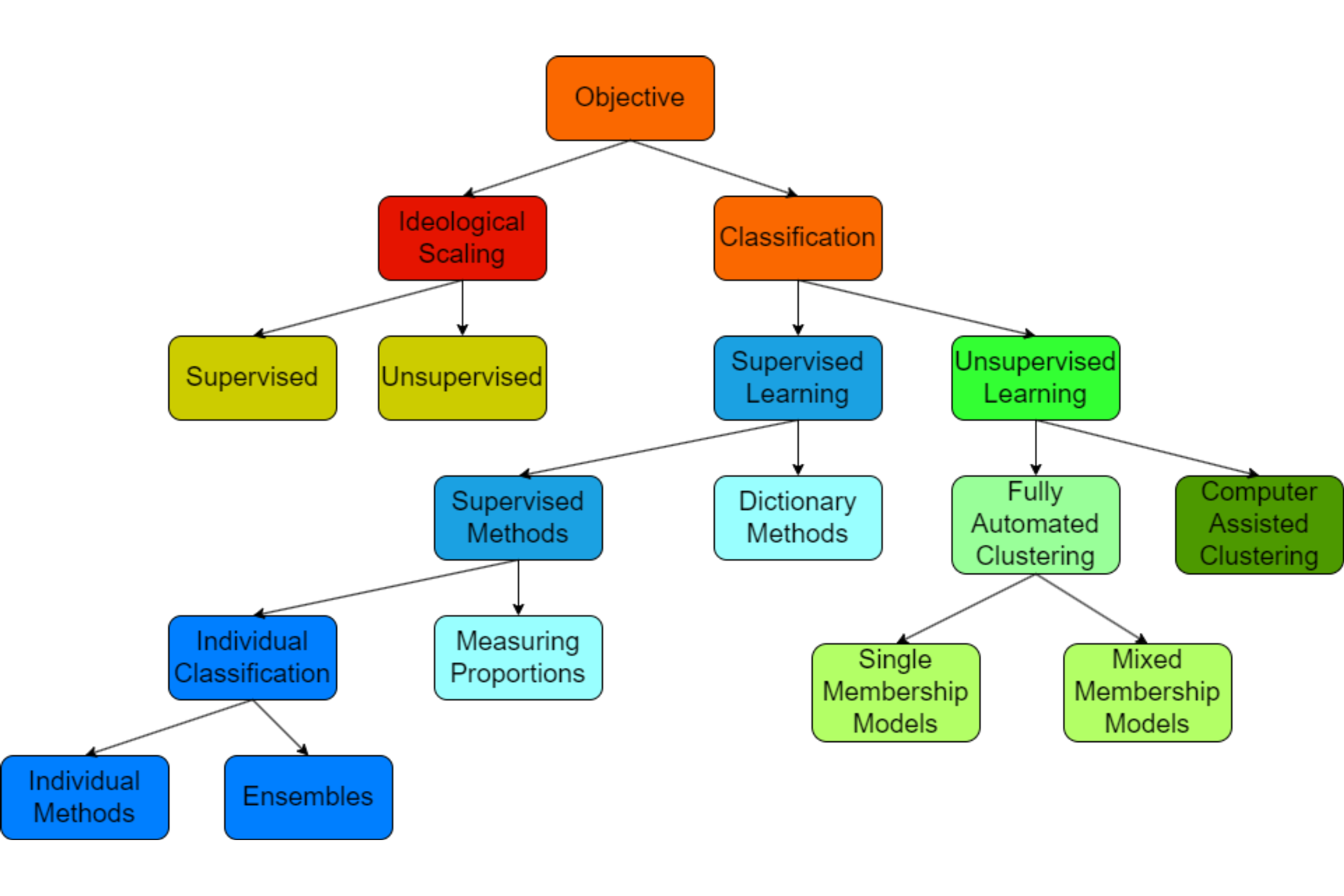
Figure 8.1: Text modeling framework in NLP
The chart in Figure 8.1 provides a full scenario of the possible paths of modeling.93
8.1.1 General setting
Most standard text models are a form of generative probabilistic model, which requires a statistical estimation process based on optimization of a cost function. The objective of the process is to obtain a set of estimates (or estimators) that optimizes the cost (i.e. lowest cost) for a predefined loss function. The variations between a type of model to another are in:
- the choice of the loss function,
- the method of estimation,
- the type of estimators, and
- the statistical properties of the estimators.94
The formal setting for the models are as follows:95
- a word is the basic unit of discrete data, indexed by a number for each word in the vocabulary derived for the entire dataset, as \(V = ({1,2,...,K})\). This is the basic category in the data.
- a document is an ordered sequence of \(N\) word, \(w = ({w_1,w_2,...,w_N})\) where \(w\) are numbers in \(V\)
- a corpus is a collection of ordered \(M\) document, consisting of ordered word, denoted by \(d = ({d_1,d_2,...,d_M})\)
The first step for pre-processing the data involves converting the entire corpus into data. The steps are: a) tokenizing, b) create a vocabulary for the tokens present, c) create the metadata for the word, document, and corpus.
All these steps were explained in previous chapters using pre-built functions in tidytext or quanteda.
The texts, now in data format, are converted to vector representations, using the vocabulary \(V\) as its look-up table (for converting back into textual form). Notationally they are as follows:
\[C = set (D,W)\]
A form of representation of \(C\) is the Document Term Matrix (DTM) as we have seen before, and the Feature Co-occurrence Matrix (FCM) is a reduced compact form of \(C\) based on co-occurrence representation.
In statistical terms, what we have now are observations, \(w_i\), which are the individual word, and its measures are the location (observation) and its frequencies. At a higher level, the observations are \(d_j\) and its measures are the numerical representation of it, which is its score. Given the setting, then the statistical problem is set as follows:
\[F_{argmin}(\theta) = LOSS(X)\]
We want to find an estimate of \(\theta\) which minimizes the loss function. Once we obtain the estimate, called \(\hat{\theta}\), we can use it to infer and obtain the estimation. The estimation (or inference) will be numbers of probability (i.e. between 0 and 1), which are the “probability scores” based on the model.
Different text models will use different model assumptions and loss functions. We provide a concise explanation for a few choices of text models that we will use in this book.
8.1.2 Supervised and unsupervised learning methods
The major difference between the supervised and unsupervised learning method is in whether the model assumes known categories (also called labels) or unknown categories (labels) of the texts under study. We can generally categorize supervised as pre-built language models, such as the one applied in the sentiment scoring example (in Chapter 3). Unsupervised models, on the other hand, utilize a generalized process of clustering, either using an in-built process of clustering (called fully automated clustering) or in-process clustering (using some algorithms) as part of the pre-processing of the data (called computer-assisted clustering).
The latest development of the supervised versus unsupervised models involves infusion of both types into each other, which falls under the name of “headless AI”, “Unsupervised AI”. The process involves combining the steps of unsupervised learning as the start, then using the results to auto-generate the labels, which are then implied into supervised learning models.96 The main difference of the infused model is the process of labeling is entrusted to the algorithms rather than human.
Since human language is a complex subject, the performance of any models, supervised, unsupervised, or both combined is still a subject that requires in-depth studies and testing. The encouraging part is, as we study more data as they become available, by way of big data, with better and faster computing power, our ability to deal with language through computational linguistics has improved tremendously.
8.1.3 Topic modeling for Quran Analytics
In this book, we will explore a specific task in NLP called “topic modeling”. This is an unsupervised machine learning method, suitable for the exploration of textual data. The calculation of topic models aims to determine the proportionate composition of a fixed number of topics in the documents of a collection. Since it is an unsupervised machine learning method, it is useful to experiment with different parameters in order to find the most suitable parameters for our own analysis needs.
Topic Modeling often involves the following steps.97
- Read in and preprocess text data,
- Calculate a topic model using a text model (using unsupervised learning model),
- Visualize the results from the calculated model and
- Select documents based on their topic composition.
Topic modeling is an interesting aspect of NLP in the sense that, given a large amount of text data, which structures are not known offhand, and we want to extract information about the text, particularly what are the “headlines” or “themes” of the text in question. The general idea is, if a term is present in many of the sentences, in a certain particular structure, then we say that it has a high probability to be the key subject of the discussion. It implies that the word has a high probability to be in the headlines or themes, in the same way as to how we think a news headline should be. Putting it another way, given the text of news without the headlines, can we guess what the headline should be?
For Quran Analytics, we know Al-Quran is arranged in a very deterministic manner (i.e. fixed permanently), and no change has occurred to the original text. Particularly each word, from the first to the last, is arranged in verses, from the first to the last (in 6,236 verses), in Surahs, from the first to the last (in 114 Surahs). Verses represent themes (or messages) of their own, and Surahs also represent a theme or combination of themes. The themes may be repeated in various words, or verses, or various parts within the Surahs, as well as various parts of the entire Al-Quran.
To perform a thorough and complete task of uncovering themes from Al-Quran, based on translated texts, is no small feat. It should be a research subject by itself. Since the purpose of this book is to introduce the subject, we will scale it down to demonstrations of the various models and focus on a specific segment of Al-Quran, through a selected Surah, namely Surah Al-Kahf.
8.2 Unsupervised learning models
As explained earlier, unsupervised learning models assume that we do not know off-hand the labeling of the texts, such as the topics of the texts under study. Our task is to “uncover” those labels, which have a high probability to be the contents of the topics for the collection of texts.
In this section we will cover some of the well known unsupervised learning models, namely:
- Latent Dirichlet Allocation (LDA)
- Latent Semantic Analysis (LSA)
- Structural topic models (STM)
First, we will provide a quick technical brief of the models.
8.2.1 Latent Dirichlet Allocation (LDA) model98
LDA is a special class factorial multinomial probit model, conditioned on topic \(z_l\), where \(z_l\) is drawn from a Poisson distribution; and the loss function is defined as \(Dir(\alpha)\) as \(p(w_n|z_l,\beta)\), a multinomial probability over the space of \(\beta\). The Dirichlet function \(Dir\) is the defining function of the model. The function relies on a method of sampling, which is pre-determined as part of the modeling process. In most applications, the standard method is “Gibbs” sampling.99
The performance of LDA has shown promising results in various applications, in particular for topic modeling on some challenging aspects, such as in information extraction from text records, social media sentiment or aspect mining, and others.100
In our work here, we will use the topicmodels package, which contains the LDA() function.
8.2.2 Structural Topic Models (STM)
The foundation of STM is provided by (M. E. Roberts et al. 2014) and developed as an R package, stm (M. Roberts et al. 2020), details of which are provided in its package article (M. Roberts, Stewart, and Tingley 2019) and its webpage guide.101
STM uses a Generalized Linear Model (GLM) framework by incorporating document meta-data into the topic modeling process. The process follows the same approach of LDA, where it is conditioned on topic \(z_l\). \(z_l\) is drawn from a Logistic Normal; and the loss function is defined as \(p(w_{d,n}|z_{d,l},\beta_{d,k=z_{d,n}})\), a multinomial probability over the space of \(\beta\). The structure is the same, but with different assumptions of conditionality and probability distributions of LDA.
In our work here, we will use the stm package, which contains many neat functions for visualization of the results.
8.2.3 Latent Semantic Analysis model
LSA was first introduced by (Landauer, Foltz, and Laham 1998) and has been around a bit longer than LDA and STM. The objective of LSA is to replicate the human cognitive phenomena using a statistical learning model. It assumes that word-for-word, word-sentence (or passage), sentence(or passage)-for-sentence (or passage) relations are correlated in the way of association or semantic similarity, within textual data.
The statistical process of LSA involves applying Single Value Decomposition (SVD) to the text matrix data (such as a DFM or DTM); from which it generates a new orthogonal space of factor values (based on the dimensions, which are the number of topics - a dimension reduction process). In the current time, the process has a resemblance to a Neural Network (for those who are familiar with it) - which is a non-parametric method of performing simultaneous multiple regression equations, and the final results will be a correlation matrix for the topics and the texts (and sentences).102
In our work here, we will use the quanteda.textmodels function called textmodel_lsa().
8.2.4 Labeling the data
We will use Surah Al-Kahf as our text under study. We choose the Surah for a particular reason; it is a medium length Surah, containing six rather distinct sections:
- the story of the cave dwellers (v1-v31),
- the story of two garden owners (v32-v44),
- a parable of worldly life (v45-v59),
- the story of Prophet Moses and Al-Khidh (v60-82),
- the story of Dhul-Qarnayn (v83-102), and
- about deeds (v103-v110).
Based on the observation, we will label the verses according to our own interpretation and investigate the subject as we go along, first using unsupervised learning, then supervised learning. In unsupervised learning, we will use the labels as a check between the model against our assumption; and in the supervised model, we will use the model to check its accuracy, against what we assume as the actual situation.
quran_all = read_csv("data/quran_trans.csv")
kahf <- quran_all %>% filter(surah_title_en == "Al-Kahf") %>%
                mutate(Group = ifelse(ayah %in% 1:31, "cave",
                               ifelse(ayah %in% 32:44, "garden",
                               ifelse(ayah %in% 45:59, "life",
                               ifelse(ayah %in% 60:82, "moses",
                               ifelse(ayah %in% 83:102, "dhul",
                               "deeds"))))))
dfm_kahf <- kahf$saheeh %>%
    tokens(remove_punct = TRUE) %>%
    tokens_tolower() %>%
    tokens_remove(pattern = stop_words$word, padding = FALSE) %>% dfm()
8.2.5 Latent Dirichlet Allocation (LDA)
We will start with the most common algorithm for topic modeling, namely Latent Dirichlet Allocation (LDA). LDA is guided by two principles.
- Every document is a mixture of topics. We imagine that each document may contain words from several topics in particular proportions. For example, in a two-topic model, we could say “Document 1 is 80% topic A and 20% topic B, while Document 2 is 40% topic A and 60% topic B.”
- Every topic is a mixture of words. Importantly, words can be shared between topics; a word like “deeds” might appear in both equally.
LDA is a mathematical method for estimating both of these at the same time: finding the mixture of words that are associated with each topic, while also determining the mixture of topics that describes each document.
For parameterized models such as LDA, the number of topics \(k\) is the most important parameter to define in advance. How an optimal \(k\) should be selected depends on various factors. If \(k\) is too small, the collection is divided into a few very general semantic contexts. If \(k\) is too large, the collection is divided into too many topics of which some may overlap and others are hardly interpretable.
For our analysis, we choose a thematic “resolution” of \(k = 6\) topics. In contrast to a resolution of 100 or more, 6 topics can be evaluated qualitatively very easily. We also set the seed for the random number generator to ensure reproducible results between repeated model inferences.
We use the LDA() function from the topicmodels (Grün et al. 2020) package, setting \(k = 6\), to create a six-topic LDA model. Almost any topic model in practice will use a larger k, but we will soon see that this analysis approach extends to a larger number of topics. The function returns an object containing the full details of the model fit, such as how words are associated with topics and how topics are associated with documents.
We need to “clean” the Document Feature Matrix, dfm from empty rows and run the LDA() function as shown below:
require(topicmodels)
drop <- NULL
for(i in 1:NROW(dfm_kahf)){
     count.non.zero <- sum(dfm_kahf[i,]!=0, na.rm=TRUE)
     drop <- c(drop, count.non.zero < 1)
   }
dfm_kahf_clean <- dfm_kahf[!drop == TRUE,]
k <- 6
lda_kahf <- topicmodels::LDA(dfm_kahf_clean, k, method="Gibbs",
            control=list(iter = 300, seed = 1234, verbose = 25))
Depending on the size of the vocabulary, the collection size, and the number \(k\), the inference of topic models can take a long time. This calculation may take several minutes. If it takes too long, reduce the vocabulary in the DTM by increasing the minimum frequency in the previous step.
The topic model inference results in two (approximate) posterior probability distributions: a distribution theta over k topics within each document and a distribution \(\beta\) over V terms within each topic, where V represents the length of the vocabulary of the Surah (V = 240).
We take a look at the 7 most likely terms within the term probabilities \(\beta\) of the inferred topics.
library(tidytext)
kahf_topics <- tidy(lda_kahf, matrix = "beta")
kahf_top_terms <- kahf_topics %>%
  group_by(topic) %>%
  top_n(7, beta) %>%
  ungroup() %>%
  arrange(topic, -beta)

kahf_top_terms %>%
  mutate(term = reorder_within(term, beta, topic)) %>%
  ggplot(aes(beta, term, fill = factor(topic))) +
  geom_col(show.legend = FALSE) +
  facet_wrap(~ topic, scales = "free") +
  scale_y_reordered()+
  theme(strip.background = element_rect(color = "black"))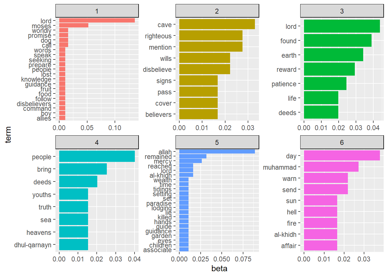
Figure 8.2: Top terms with LDA methods for Surah Al-Kahf
From Figure 8.2 we can see that the first topic contains the term “moses” and the second topic contains “cave”, and so on along the lines of the six topics we assumed. However, we see the various terms are mixed within the topics. As an example, the term “al-khidh” appears in a few of the top terms in two of the topics, and various other terms crisscrossing among the topics.
The reason why terms can be mixed between topics, despite we assuming that it shouldn’t happen (for example we know precisely that “al-khidh” appears only in the specific segment), is due to the fact that the model does not “know” the topics off-hand. It only assumes six topics which location within the texts is assumed to be of equal probability across the entire text. What LDA does is to coerce six dimensions onto the data and figure out how best the six dimensions “fit” the data. Whatever the outcome is the result of this process.
Furthermore, LDA tries to generate a pecking order for the topics, by giving one of the dimensions (i.e. topic) the highest rank from any of the six possibilities, followed by the second dimension and so forth. We can check which topics have a “higher” hierarchical clustering by checking its similarity using a distance method (as explained in Chapter 7), such as a Euclidean distance.103
lda.similarity <- as.data.frame(lda_kahf@beta) %>%
  scale() %>%
  dist(method = "euclidean") %>%
  hclust(method = "ward.D2")
plot(lda.similarity, xlab = "")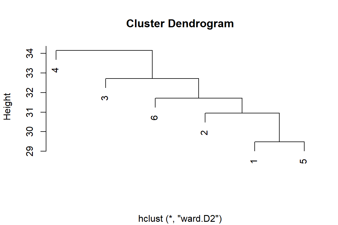
Figure 8.3: LDA topic similarity by features for Surah Al-Kahf
From Figure 8.3, we can say that the topic at the highest level is Topic 4, followed by Topic 3, Topic 6, Topic 2, and finally Topic 1 and Topic 5.
Let’s take topic 4 as our sample (being the highest rank) and put the terms into a sentence as follows:
people - bring - deeds - youths - truth - sea - heavens - dhul-qarnayn
This is a typical output of text modeling exercise, where grammatically and semantically the subjects are necessarily clear for a reader. A careful reading of the text shows that the top terms within any topic do not follow exactly what we got from the text (i.e. the Saheeh translation of the Surah). Why this is the case, is a clear example of what has been noted by linguists, as “grammar leaks”, which in essence means that grammars are not easily captured within a textual analysis. This issue is particularly notable when we use most of the unsupervised learning methods, such as the LDA.
8.2.6 Structural Topic Models (STM)
Let us look at an alternative method dealing with topic modeling, namely stm or Structural Topic Models.
library(stm)
dfmkahf_stm <- quanteda::convert(dfm_kahf, to = "stm")
stm_kahf <- stm(
  dfmkahf_stm$documents,
  dfmkahf_stm$vocab,
  K = 6,
  data = dfmkahf_stm$meta,
  init.type = "Spectral"
)
We can view the results of the model using the following codes:
We can see from the output that there four different statistics which can be used to rank the terms for a topic; the highest probability, FREX (frequency), Lift, and Score. Different terms will rank higher if we use different measures and the ranking also changes with the measures. What we want to emphasize is that the “curse of dimensionality” is a major issue which we face in these types of analyses.
Let us plot the top words in topics:
kahf_topics2 <- tidy(stm_kahf, matrix = "beta")
kahf_top_terms <- kahf_topics2 %>%
  group_by(topic) %>%
  top_n(7, beta) %>%
  ungroup() %>%
  arrange(topic, -beta)

kahf_top_terms %>%
  mutate(term = reorder_within(term, beta, topic)) %>%
  ggplot(aes(beta, term, fill = factor(topic))) +
  geom_col(show.legend = FALSE) +
  facet_wrap(~ topic, scales = "free") +
  scale_y_reordered()+
  theme(strip.background = element_rect(color = "black"))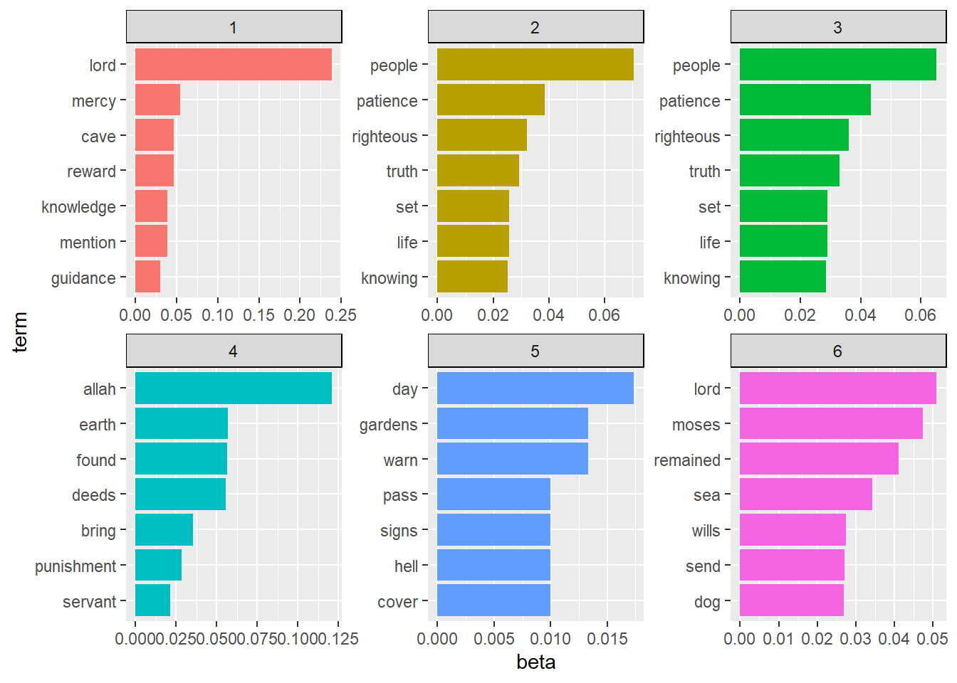
Figure 8.4: STM topic shares for Surah Al-Kahf
We can see, from Figure 8.4 that STM brings different results compared to LDA. Which one is more accurate, is impossible to tell from the results. We can produce the same hierarchical plot as we did for the LDA as follows:
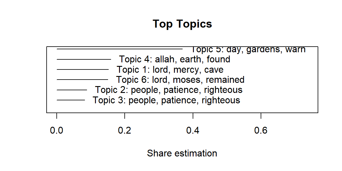
Figure 8.5: STM topic shares for Surah Al-Kahf
Figure 8.5 and the results for top-words in Figure 8.4 demonstrate clearly that STM methods apply a different dimensionality reduction approach than the LDA. From the plot of share estimation in Figure 8.5, about 45% of the texts are explained by Topic 5, followed by about 16% by Topic 1 and Topic 6.
There are few other neat options within STM that are useful and we will demonstrate them here. One of the functions is findThoughts(), which is a tool to find the subjects of a topic within the texts. We will try to get two verses in which Topic 5 and Topic 2 are dominant, as a sample:
thoughts4 = findThoughts(stm_kahf, n = 2,text = kahf$saheeh[1:107],
                         topics = 5)$docs[[1]]
thoughts3 = findThoughts(stm_kahf, n = 2,text = kahf$saheeh[1:107],
                         topics = 2)$docs[[1]]
par(mfrow = c(1, 2),mar = c(.5, .5, 1, .5))
plotQuote(thoughts4, width = 45, main = "Topic 5")
plotQuote(thoughts3, width = 45, main = "Topic 2")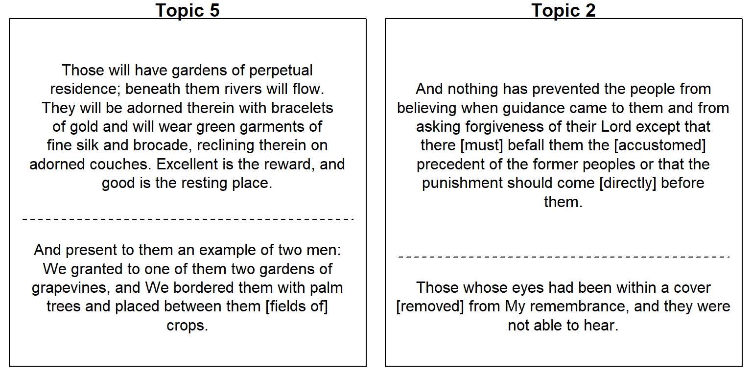
Figure 8.6: Sample of verses highly associated with Topic 5 and Topic 2
We present the results in a wordcloud format in Figure 8.7.
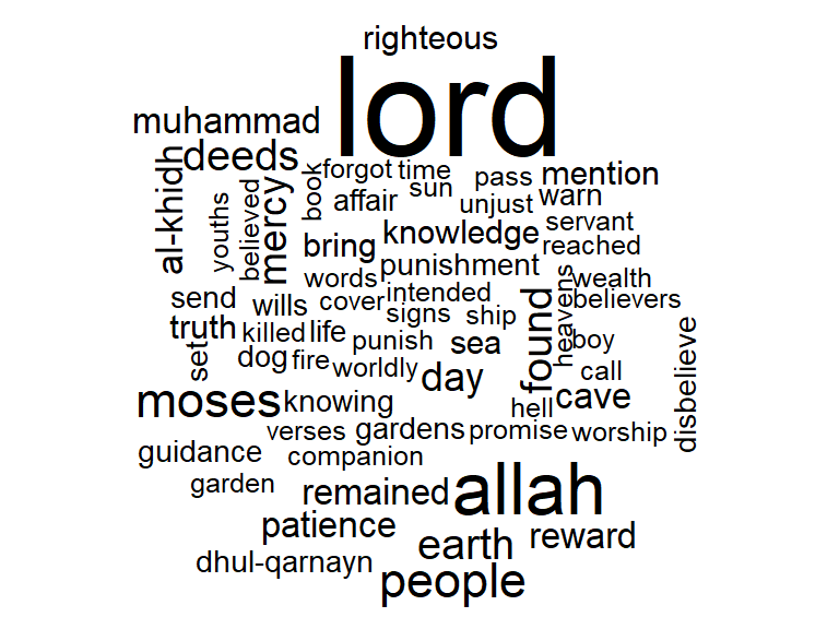
Figure 8.7: Top words from all topics in wordcloud from STM for Surah Al-Kahf
We can visualize the correlations between the topics in Figure 8.8:
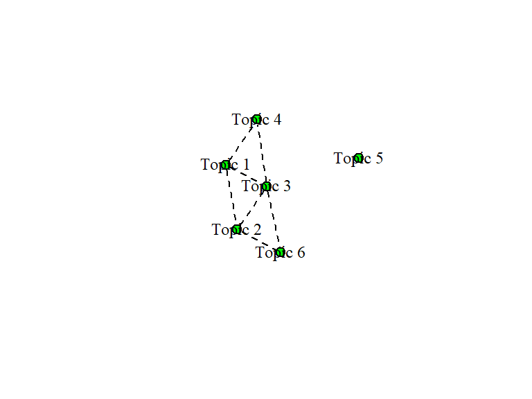
Figure 8.8: Graphical display of topic correlations from STM for Surah Al-Kahf
Figure 8.9 is a perspective comparison between the lowest share estimate, Topic 2, against the highest, Topic 5.
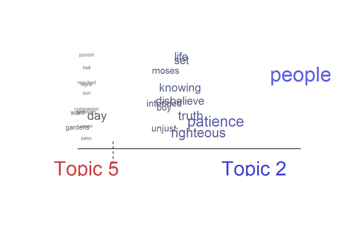
Figure 8.9: Two perspective for topics from STM in Surah Al-Kahf
Figure 8.9 shows that all that the computer sees are numbers and their dimensions (i.e. model); where all the texts are represented by probabilities (by the sizes of the texts) and distances (by positions of the texts). It is not easy to convert these numbers and dimensions into a humanly readable format.
The important thing to note is that these models take words in the texts as “they are”, without altering their positions (except for stopwords removals) and capture their occurrences. From there on, the models apply statistical calculations based on the formula provided within the models. Statistically speaking, the results are how the data “speak for itself”. The exact meanings are for the human to interpret.
The table below provides top-terms to top-terms comparison from both the STM and LDA results, by ranking order.
| Topic | STM |
|---|---|
| Rank 1 | (Topic 5) allah, day, muhammad |
| Rank 2 | (Topic 1) lord, earth, mercy |
| Rank 3 | (Topic 6) people, cave, sea |
| Rank 4 | (Topic 4) deeds, found, remained |
| Rank 5 | (Topic 3) moses, righteous, life |
| Rank 6 | (Topic 2) moses, righteous, guidance |
| Topic | LDA |
|---|---|
| Rank 1 | (Topic 4) people, bring, deeds |
| Rank 2 | (Topic 3) lord, found, earth |
| Rank 3 | (Topic 6) day, muhammad, warn |
| Rank 4 | (Topic 2) cave, righteous, mention |
| Rank 5 | (Topic 1) lord, moses, worldly |
| Rank 6 | (Topic 5) allah, remained, mercy |
We can see the impact of text entropy on the results, where the method choice changes the outcome dramatically. Not only does the topic change its ranking, but the terms also change its ranking within a topic and across topics.
8.2.7 Latent Semantic Analysis (LSA)
Latent Semantic Analysis is said to be better at capturing the “semantical” elements within the texts (Landauer, Foltz, and Laham 1998). We will see the results and compare them to the STM and LDA methods earlier.
First, let us explain the approach of LSA. There are two different methods of vectorization which we can utilize: vectorization over the features (similar to LDA and STM) or vectorization over the verses. Both have their advantages and disadvantages, depending on our objective. For our purpose, we will do both, first by the features method, so that we can compare the results with STM and LDA. In both methods, we fix the number of topics to be six, by setting nd = 6 (six dimensions).
LSA works by calculating every individual word within the texts, it computes the score of a sentence (i.e., verses) in the texts, and computes the “distances” between the sentences (verses). These distances are captured through the dimensions of vectorized space of six dimensions (since we chose six topics as our target). The top words for each topic (i.e. dimensions) are the headers as printed above.
Comparing with previous results from STM, LDA:
| Topic | STM |
|---|---|
| Rank 1 | (Topic 5) allah, day, muhammad |
| Rank 2 | (Topic 1) lord, earth, mercy |
| Rank 3 | (Topic 6) people, cave, sea |
| Rank 4 | (Topic 4) deeds, found, remained |
| Rank 5 | (Topic 3) moses, righteous, life |
| Rank 6 | (Topic 2) moses, righteous, guidance |
| Topic | LDA |
|---|---|
| Rank 1 | (Topic 4) people, bring, deeds |
| Rank 2 | (Topic 3) lord, found, earth |
| Rank 3 | (Topic 6) day, muhammad, warn |
| Rank 4 | (Topic 2) cave, righteous, mention |
| Rank 5 | (Topic 1) lord, moses, worldly |
| Rank 6 | (Topic 5) allah, remained, mercy |
| Topic | LSA |
|---|---|
| Rank 1 | (Topic 1) lord, allah, mercy |
| Rank 2 | (Topic 5) adorned, resting, wills |
| Rank 3 | (Topic 6) wills, truth, disbelieve |
| Rank 4 | (Topic 4) allah, cave, guide |
| Rank 5 | (Topic 3) people, lord, mercy |
| Rank 6 | (Topic 2) lord, words, righteous |
To see how this looks, we plot the sentences scoring for each verse (denoted by the number), and across dimensions (we chose dim1 vs dim2, and dim1 vs dim 3, for illustration). Sentences that are “semantically” closer based on “topic a” vs “topic b” are clustered together. This is shown in Figure 8.10.
Name = str_replace(rownames(klsa_df),"text","")
p1 = klsa_df %>% ggplot(aes(x = V1, y = V2), label= Name) +
  geom_point(size = 2, alpha = 0.6, color = verses.color) +
  theme_bw()+
  geom_text(aes(label=Name,hjust=1, vjust=1))
p2 = klsa_df %>% ggplot(aes(x = V1, y = V3), label= Name) +
  geom_point(size = 2, alpha = 0.6, color = verses.color) +
  theme_bw()+
  geom_text(aes(label=Name,hjust=1, vjust=1))
cowplot::plot_grid(p1,p2, nrow = 1)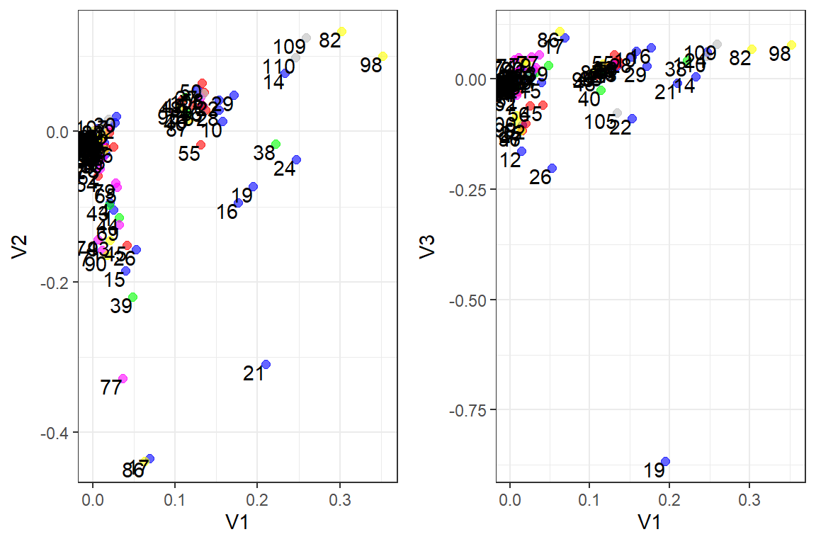
Figure 8.10: Topics in dimensions for Surah Al-Kahf
In Figure 8.10, there are (supposed to be) six groupings of dimensions (which are topics). Semantically, we can see that on Topic 1 and Topic 2, as well as Topic 1 and Topic 3, the groupings and the distances between the groupings are not as clear and lumpy in nature. This is due to the fact that we “force” the number of topics to be six by choice. This is the problem of choosing parameters for the model because it dictates the final results based on the assumptions we use.
Now let us present the results from another perspective, that is to view the scores for the topics across the verses. Since it is not easy for us to print the scores and visualize them, we plot the scores in a 3D plotter and present the plot output in Figure 8.11.
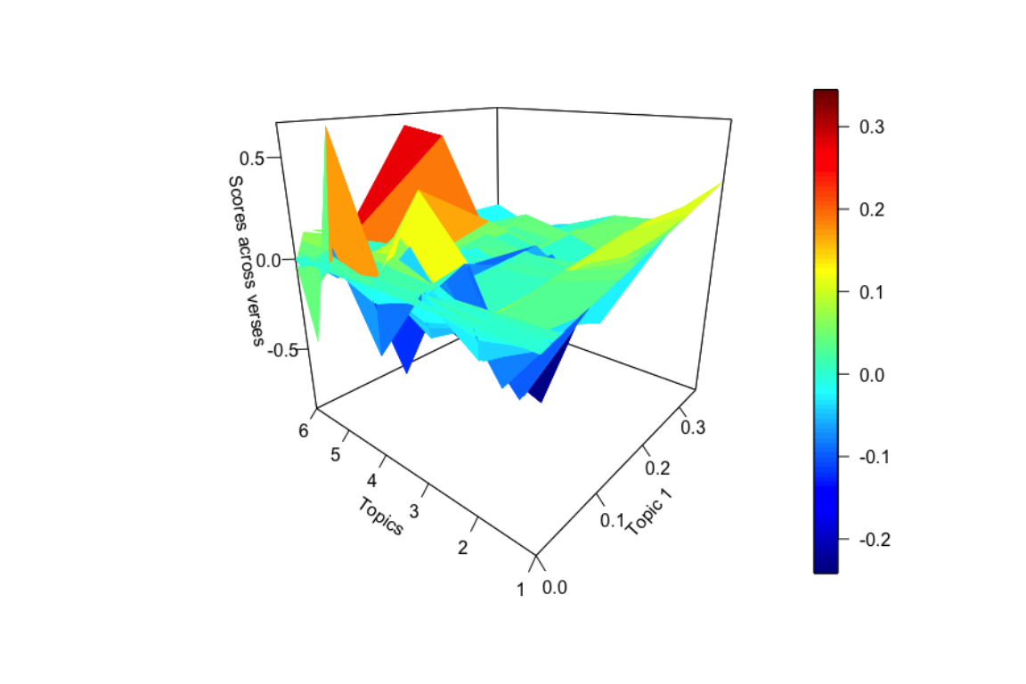
Figure 8.11: 3D plot of the scores from LSA model for topics in Surah Al-Kahf
The plot shows that for Topic 1 (the highest-ranked topic), there are verses that have high positive scores. For Topic 5 and Topic 6, almost similar verses have high positive scores, while for Topic 3, the scores are highly opposite (i.e. negative) on some of the verses. This is not exactly the ideal method to extract the information from the model, since visualization of the complex dimensionality is not easy and clear. However, what we want to demonstrate is there are deeper level complexities that are not easy to identify by just eyeballing the visuals.
8.2.8 Summarizing unsupervised learning model
Let us summarize the lessons learned from the LDA, STM, and LSA models of Surah Al-Kahf.
Firstly, we note that for the Surah Al-Kahf, we have 507 unique tokens (or vocabulary) from 110 documents (verses), which means that the matrix of data space of 55,770 observations (507 x 110), which is a sparse matrix of 0’s and 1’s. In the examples we went through, we are trying to estimate 3,549 parameters ((6+1) x 507). Statistically, we are facing an extremely small data set (due to sparsity) while trying to estimate a large number of parameters. This is the first part of the problem we are facing.
Secondly, we need to mention a few notable problems. Is it justified to assume that words, lexically and semantically follow certain patterns and structures within Saheeh English translations of Al-Quran? In the English language, there are abundant works by linguists to deal with this issue. However, if the texts are translations from another language, which has its own grammatical, lexical, and semantical meaning, does the same thing hold? Naturally, the answer is not necessarily. This is particularly true for Quran Analytics since the narratives, stories, and expositions in Al-Quran are explicit and not in the normal human linguistic way.
Summarizing the observations and results of the LDA, STM, and LSA models, we can generally say that the unsupervised learning model represented by the three, despite the sparse data situation, performed reasonably well in capturing some elements in the structure of the texts from statistical perspectives. The model variations could very well result from a small sample problem.
Generally, we would say that, if more analysis is done, like, instead of relying on a single Surah (as we have done here), we could use the entire corpus of Saheeh, and augment the data with other translations (Yusuf Ali and other English translations available). This may help deal with the small sample/data problem. Furthermore, if data augmentation involves the original Arabic text combined with some refinement of the modeling approach, we believe that some interesting insights are possible. This is the more comprehensive Quran Analytics approach that we target. For now, we leave the subject as directions for future research.
8.3 Supervised learning models
A supervised learning model requires two sets of data, the training sample and the validation sample. Both samples must be labeled data, where the categories are pre-labeled, obtained from some other pre-worked dataset, or the user’s own labeling. Since we have attempted to label Surah Al-Kahf with six labels (i.e., topics), we want to test some of the supervised learning models and compare the performance and results.
We will choose the simplest method, Naive Bayes (NB), followed by Support Vector Machines (SVM). We will then compare the methods at the end of this section.
First, we create the labels for the data and split the samples for training and validation set as follows:
label_index = data.frame("index" = 1:110,
                         "topics" = c(rep("cave",(31-1+1)),
                                      rep("garden",(44-32+1)),
                                      rep("life",(59-45+1)),
                                      rep("moses",(82-60+1)),
                                      rep("dhul",(102-83+1)),
                                      rep("deeds",c(110-103+1))))
train_index = sample(label_index$index,55)
kahf_full = data.frame("text" = kahf$saheeh, "label"= label_index$topics)
kahf_train = kahf_full[train_index,]
kahf_valid = kahf_full[-train_index,]
label_train = kahf_train$label
label_valid = kahf_valid$label
dfm_train = kahf_train$text %>% tokens(remove_punct = T) %>%
                tokens_tolower() %>%
                tokens_remove(pattern = stop_words$word, padding = F) %>%
                dfm()
dfm_valid = kahf_valid$text %>%  tokens(remove_punct = T) %>%
                tokens_tolower() %>%
                tokens_remove(pattern = stop_words$word, padding = F) %>%
                dfm()
8.3.1 Naive Bayes (NB)104
The Naive Bayes model for text classification is a simple “Bag-of-Words” model, where we assume a (prior) multinomial probability for six topics, which we assume by default. Each verse is assumed to have an equal probability of belonging to a topic. The model then will calculate the probability of a verse belonging to any one of the topics. By default, we know which verses are from which topics, as defined in the six labels that we have set before.
The Naive Bayes model in quanteda is simply fitted and tested as follows:
nb_kahf = quanteda.textmodels::textmodel_nb(dfm_train,label_train)
table1 = table(predict(nb_kahf),label_train)
table1
dfm_matched <- dfm_match(dfm_valid, features = featnames(dfm_train))
pred = predict(nb_kahf, newdata = dfm_matched)
table2 = table(pred, label_valid)
table2
We can see from the results in the confusion matrix table, table1, that in the training set, the Naive Bayes model has a perfect fit (almost all correct matches) with the accuracy of 100%. However, when fitted with the balance of the data (validation data), there are several mismatches, and the accuracy drops down to 50.91%. We have an overfitting problem.
8.3.2 Support Vector Machines (SVM)
Support Vector Machines or SVM is among the basic multivariate regression models which are based on separating hyperplanes concept. The idea of SVM is to generate classifications across multi-labels by separating the data into separate “planes” of classes.
In quanteda, the model can be applied using textmodel_svm() function.
svm_kahf = quanteda.textmodels::textmodel_svm(dfm_train,label_train, weight = "uniform")
table3 = table(predict(svm_kahf),label_train)
table3
pred = predict(svm_kahf, newdata = dfm_matched)
table4 = table(pred, label_valid)
table4
We can see from the results of the table that in the training set, the SVM model fits with an accuracy of 100%. However, when fitted with the balance of the data (validation data), there are several mismatches, and the accuracy is at 4545%. It suffers the same problem as the Naive Bayes model, which is an overfitting problem.
8.3.3 Summarizing supervised learning model
Our excursion on the supervised learning model is very short, with unsatisfactory results. The problem we face is quite obvious, namely small sample data. We have only a few verses for each topic, and within each topic, we have only a small number of features. When we fit the model, it will easily get overfitted, which to a degree says that our labeling of the verses is precise within its own dataset whereby the model would detect it easily. However, we can never use the learned model to apply to verses beyond the actual training sample, which then renders the exercise practically useless.
8.4 Ideological difference models
quanteda.texmodels has a few other supervised learning models, such as textmodel_wordscores() and textmodel_wordfish(). Both models are useful for observing the “ideological” differences in texts. The concept of both models is to uncover if there are any differences ideologically speaking between the various topics. If there are “distinct” ideas, the model should be able to predict them. These types of models are in the category of “ideological scaling”, a supervised learning model (please see Figure 8.1) at the beginning of the chapter.
First, we will apply the wordscores model in the codes attached below, and tabulate the results.
ws_kahf = textmodel_wordscores(dfm_train,
                               y = as.numeric(as.factor(label_train)))
table5 = table(floor(predict(ws_kahf)),
               as.numeric(as.factor(label_train)))
table5
table6 = table(floor(predict(ws_kahf, newdata = dfm_matched)),
               as.numeric(as.factor(label_train)))
table6
From the tables printed above, we can say that in the training part (table5), the model could clearly identify that the “ideas” within each topic are distinct enough to be detected with the accuracy of 38.18%. In table6, when we apply the model to the validation data, we can see that some of the topics (ideas) are dispersed through other topics (ideas).
textplot_scale1d(ws_kahf, margin = "features",
                 highlighted = c("allah","lord","moses","cave",
                                 "al-khidh","gardens"),
                 highlighted_color = "darkred")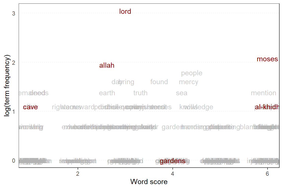
Figure 8.12: Wordscores plot for Surah Al-Kahf
Now we will plot the scores from the model together with some words to be highlighted. The plot is shown in Figure 8.12. From the plot we can visualize the relative positions of the key words for the various topics: “lord”, which rank highest in the Surah, followed by “allah” - both almost at the center; the word “moses” scores higher, but in the same “direction” as “al-khidh”, which is directly below “moses”. The word “cave” and “gardens” are figuratively apart. Similar exercises can be performed for various selections of key terms and we can observe its relative position within the whole text.
Now we will apply textmodel_wordfish(), which in many ways, similar to wordscores model and plot the results.
wf_kahf = textmodel_wordfish(dfm_train, dir = c(1,2))
textplot_scale1d(wf_kahf, margin = "features",
                 highlighted = c("allah","lord","moses","cave",
                                 "al-khidh","gardens"),
                 highlighted_color = "darkred")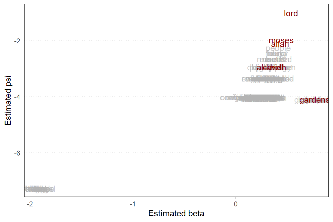
Figure 8.13: Wordfish plot for Surah Al-Kahf
wordfish scores which will show whether some of the topics are “diametrically” opposed to one another. Figure 8.13 demonstrates that all topics are pretty much “aligned” to each other from the word “lord”, down to “gardens”. An interesting observation is that “moses” is right after “lord” in the ranking, above “allah”.
8.5 Word embeddings models
In this section we will introduce a powerful approach to dealing with text data, using a text embedding method known famously as GloVe: Global Vectors for Word Representation (Pennington, Socher, and Manning 2014). It is “an unsupervised learning algorithm for obtaining vector representations for words”. The concept of word-vector representations is to develop a global word-word co-occurrence matrix that tabulates how frequently words co-occur with another one in a given corpus.105 The model first sets a pre-training on all the data within the corpus, allowing any utilization thereafter to be easy and fast.
Mathematically what the GloVe algorithm does is to transform the corpus into a “flat” and “compact” matrix of features (row-wise) vectors. Each feature is represented as a vector of fixed length (known as the dimension) set by the algorithm. The concept is similar to hashing algorithms, where each vector is unique (representing a unique feature or word in the vocabulary). Normally the length of the vector is set to fifty, which is deemed to be sufficient for most large-size tasks. We introduce the concept here for purposes of illustrating the usage and convenience of the algorithm and demonstrate its potential for Quran Analytics.
In R, the GloVe algorithm is implemented through the text2vec (Selivanov, Bickel, and Wang 2020) package.
The steps in text2vec are as follows:106
- space_tokenizer() and itoken() for tokenization of the corpus or texts, which includes any removal of unwanted items (stopwords, punctuations, etc.)
- create_vocabulary() to create the vocabulary for the entire tokens (i.e. unique tokens)
- vocab_vectorizer() to vectorized the vocabulary
- create_tcm() to create the term-co-occurrence-matrix (tcm) and set the skip grams window
- GlobalVector$new() to generate the matrix of vectors for each vocabulary item, and set the length of the vector (to 50)
- xxx$fit_transform() to fit the GloVe model
- Use the model to predict
Note that the package uses data.table syntax for data.frame, which is an extremely fast data processor in R.
## load the library
library(text2vec)
## clean the texts
quran_saheeh = tolower(quran_all$saheeh)
quran_saheeh = gsub("[^[:alnum:]\\-\\.\\s]", " ", quran_saheeh)
quran_saheeh = gsub("\\.", "", quran_saheeh)
quran_saheeh = trimws(quran_saheeh)
## 1. tokenize
ktoks = space_tokenizer(quran_saheeh)
itktoks = itoken(ktoks, n_chunks = 10L)
stopw = stop_words$word
## 2. create vocabulary
kvocab = create_vocabulary(itktoks, stopwords = stopw)
## 3. vectorize the vocabulary
k2vec = vocab_vectorizer(kvocab)
## 4. create the tcm
ktcm = create_tcm(itktoks, k2vec, skip_grams_window = 5L)
## 5. generate the Global Vector with rank = 50L
kglove = GlobalVectors$new(rank = 50, x_max = 6)
## 6. Fit the GloVE model
wv_main = kglove$fit_transform(ktcm, n_iter = 20)
## Use the model for prediction
wv_context = kglove$components
## This is in data.table format
word_vec = wv_main + t(wv_context)
## This is to convert to dplyr data.frame format
word_vec_df = as.data.frame(t(word_vec))
The word-vector consists of vectors of unique frequencies for each word in the vocabulary. These frequencies are used for calculating the similarities or distances between the words. A plot of selected word frequencies in the word-vector is presented in Figure 8.14, for the word “allah”, “lord”, “muhammad”, and “abraham”.
word_vec_df %>% ggplot() + geom_line(aes(x=1:50, y=allah), color = "red") +
                    geom_line(aes(x=1:50, y=lord), color ="steelblue") +
                    geom_line(aes(x=1:50, y=muhammad), color = "magenta") +
                    geom_line(aes(x=1:50, y=abraham), color = "green") +
                    labs(x = "Dimensions", y = "Word Frequencies")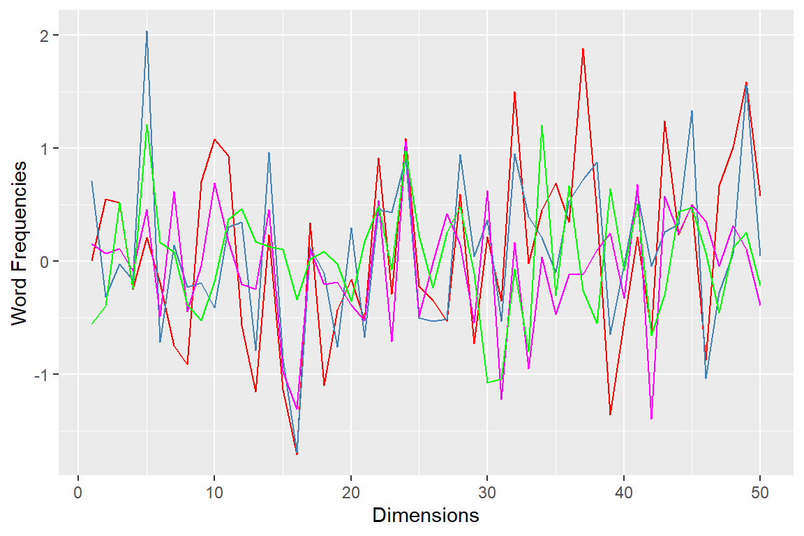
Figure 8.14: Word-vector frequencies for selected words
The frequencies do not have any meaning, except that it records the relative unique position of each word within a corpus. This method is a faster way of generating an unsupervised learning model for the data at hand, especially when the data (i.e., text corpus) is large and sparse.107
The codes below show some examples of how the GloVe model is used.
topic1 = word_vec["allah",,drop = FALSE] +
         word_vec["lord",,drop = FALSE] +
         word_vec["muhammad",,drop = FALSE] +
         word_vec["abraham",,drop = FALSE]
topic1_sim = sim2(x = word_vec, y = topic1, method = "cosine")
head(sort(topic1_sim[,1], decreasing = T),7)
Now we can see clearly the topical relevance of the words by rank, from “lord”, to “allah”, then “muhammad”, as a “messenger”, bringing the “truth” to be “believed” by the “people”, and so on. The word “abraham” (Prophet Ibrahim a.s.) appears much further down in the ranking.
Now instead of us “fixing” the topics as in the LDA, STM, and LSA to six topics, we can use the words we think are relevant for the topic and observe the results. Let us imagine the story of the cave dwellers in Surah Al-Kahf, and try to pick out “cave” and “dwell” from the entire translation.
topic = word_vec["cave",,drop = FALSE] + word_vec["dwell",,drop = FALSE]
topic_sim = sim2(x = word_vec, y = topic, method = "cosine")
head(sort(topic_sim[,1], decreasing = T),7)
As an exercise, let us look at “worship”,“allah” and “idols”.
tt = word_vec["worship",,drop = FALSE] + + word_vec["allah",,drop = FALSE]
tt_sim = sim2(x = word_vec, y = tt, method = "cosine")
head(sort(tt_sim[,1], decreasing = T),7)
tt = word_vec["worship",,drop = FALSE] + + word_vec["idols",,drop = FALSE]
tt_sim = sim2(x = word_vec, y = tt, method = "cosine")
head(sort(tt_sim[,1], decreasing = T),7)
Let us now go back to Surah Al-Kahf and redo the topic modeling exercise but instead, we will use the GloVe formulations and set the topic to be six (the same as before).
kahf_saheeh = quran_all %>%
                  filter(surah_title_en=="Al-Kahf") %>%
                  pull(saheeh)
kahf_saheeh = tolower(kahf_saheeh)
kahf_saheeh = gsub("[^[:alnum:]\\-\\.\\s]", " ", kahf_saheeh)
kahf_saheeh = gsub("\\.", "", kahf_saheeh)
kahf_saheeh = trimws(kahf_saheeh)
tokens = word_tokenizer(kahf_saheeh)
it = itoken(tokens, ids = 1:length(kahf_saheeh),
            progressbar = FALSE)
stopw = stop_words$word
v = create_vocabulary(it,stopwords = stopw)
v = prune_vocabulary(v,
                     term_count_min = 3,
                     doc_proportion_max = 0.2)
vectorizer = vocab_vectorizer(v)
dtm = create_dtm(it, vectorizer, type = "dgTMatrix")
set.seed(12345)
lda_model = text2vec::LDA$new(n_topics = 6,
                              doc_topic_prior = 0.1,
                              topic_word_prior = 0.01)
doc_topic_distr =
  lda_model$fit_transform(x = dtm, n_iter = 1000,
                          convergence_tol = 0.001,
                          n_check_convergence = 25,
                          progressbar = FALSE)
Figure 8.15 shows the prominence of the topics in Surah Al-Kahf. We can see better which topics rank higher, in fact, only a few of the topics are prominent compared to others.
barplot(doc_topic_distr[1, ], xlab = "topic",
        ylab = "proportion", ylim = c(0, 1),
        names.arg = 1:ncol(doc_topic_distr))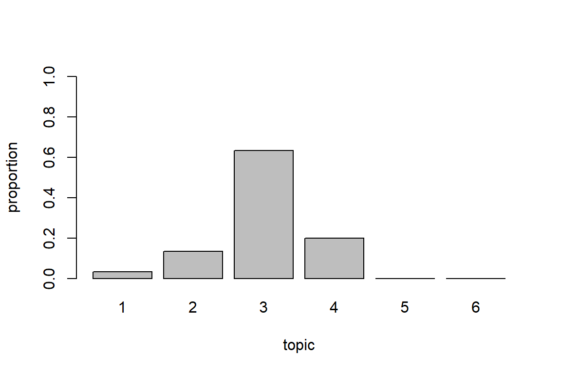
Figure 8.15: Topic bar plot for Surah Al-Kahf using GloVe model and LDA
We can get the top words for each topic, sorted by probability ranking as follows:
Without knowing what are the topics in Surah Al-Kahf, it is amazing to see that indeed the six topics can be seen from the words: cave dwellers from Topic 5, the two owners of the gardens in Topic 3, Moses and Al-Khidh in Topic 6, and Dhul Qarnayn in Topic 4.
We will fit the LSA model one more time, using the GloVe algorithm, and plot the results.
lsa_model = text2vec::LSA$new(n_topics = 6)
doc_topic_distr =
  lsa_model$fit_transform(x = dtm, n_iter = 1000,
                          convergence_tol = 0.001)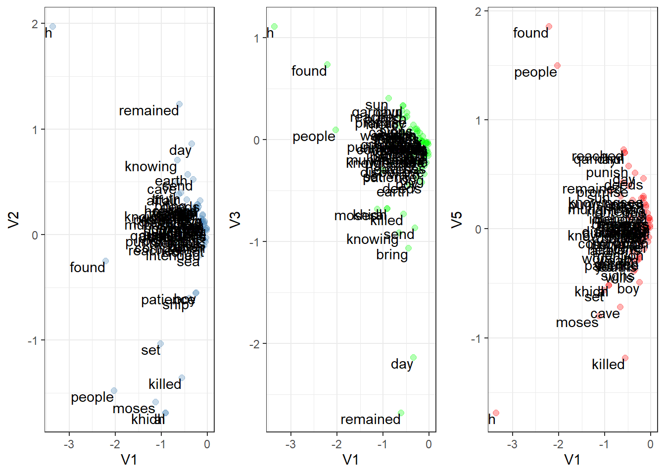
Figure 8.16: Topics in dimensions for Surah Al-Kahf using LSA and GloVe
The results in Figure 8.16 are different from the ones in Figure 8.10, where instead of the verses, we plot it over the words. As noted in many experiments using the LSA model, while it can generate distinctions between the topical relations, it is very hard to interpret the output. We can see that more “verbs” (such as “remained”, “found”, “killed”) appear to be further from the main clustering, which semantically carries more meaning than just proper nouns or names.
8.5.1 Summarizing word embedding model methods
The examples from this section on word embeddings using GloVe algorithms show promising results and demonstrate the strength of the method. It is a new generation of unsupervised learning methods for NLP tasks of finding topics, analyzing various language structures, and many others. The strength of GloVe lies in its simplicity and reliance on “closed and compact” space representations of text data, which allows us to deal with the problems of the Power Law distribution of Zipf’s law and many other statistical anomalies in text analysis. The strength of GloVe is proven by the fact that it is used heavily by Google (as it was originally developed together between Google and Stanford NLP Group).
8.6 Summary
The chapter explored the subject of text modeling by traversing through unsupervised and supervised learning models. We have demonstrated the uses and benefits of the models by applying them on topic modeling tasks applied on Surah Al-Kahf. Generally, we would say that any modeling for the English translations of Al-Quran using these models will suffer from “small sample” problems, due to sparsity structures within the data.
In the case of the supervised model, despite the shortcoming of sample size problems (i.e., model overfitting), there is still a high potential of usage if annotations and labeling are obtained correctly. These annotations are available in the form of exegesis of Al-Quran, such as the Tafseer of Ibnu Katheer and others. The annotations can be used as training labels and hence the model can be improvised to better predict the data. This is one area of future research for Quran Analytics.
On the other hand, classical and older versions of the unsupervised learning model, such as Latent Dirichlet Allocation (LDA) and Latent Semantic Analysis (LSA) are a bit arcane in the results; despite having potentials of further development along the lines forwarded by the model, conceptually. For Structural Topic Models (STM), there are many other potentials for improvements, since it has many flexibilities for changing and altering modeling assumptions.
We have not covered another large area of supervised and unsupervised learning using Neural Network models, as well as Deep Learning models of Neural Networks. Similarly, there are also powerful models based on Hidden Markov Models (HMM), which we have not covered. HMM has been extremely successful in speech recognition modeling. All these areas are very large and require extensive work for which we envisage our Quran Analytics project to undertake.
Lastly, we introduced the Word-to-Vector model of GloVe algorithms, which is an extremely useful tool with wide application potential. This is an example of a new generation of unsupervised learning models which is gaining popularity. Combining GloVe with Deep Learning is of course a venture that is among the latest in NLP research.
Since there are too many areas to cover, we end the chapter by concluding that the area of applications of text models, machine learning models (supervised and unsupervised) in Quran Analytics is just at the beginning, there are lots more to be discovered.
8.7 Further readings
quanteda package documentation (https://quanteda.io).
LDA package references from (Blei, Ng, and Jordan 2003).
LSA package references from (Landauer, Foltz, and Laham 1998).
STM package references from (M. E. Roberts et al. 2014) and (M. Roberts, Stewart, and Tingley 2019).
text2vec package references (http://text2vec.org/index.html)
GloVE references (https://cran.r-project.org/web/packages/text2vec/vignettes/glove.html)
References
Please see https://nlp.stanford.edu/projects/glove/ for details.↩︎
This is our own remake of points from (Grimmer and Stewart 2013) paper.↩︎
The basic setting is based on standard or canonical statistical inference methods.↩︎
The notations here follow (Blei, Ng, and Jordan 2003).↩︎
An example of this approach is h2o.ai, https://www.h2o.ai↩︎
For a more detailed explanation, please refer to (Blei, Ng, and Jordan 2003).↩︎
For a reference on Gibbs sampling, please see: https://en.wikipedia.org/wiki/Gibbs_sampling↩︎
A comprehensive survey of LDA model applications is provided by (Jelodar et al. 2019).↩︎
For detail exposition, please refer to (Landauer, Foltz, and Laham 1998).↩︎
Mathematically what this means is that we measure the dimensional entropy across the six possible dimensions, and rank the dimension with the highest entropy first, followed by the next.↩︎
For reference, please refer to https://quanteda.io/reference/textmodel_nb.html↩︎
The model is compiled in C++ language and wrapped into R; which provides fast speed of computation and memory-efficient processes.↩︎
Note that the matrix is a much more compact space than the DFM or FCM matrices we looked at earlier in tidytext and quanteda.↩︎