2 Word Frequency Analysis
The first task in word analytics in a corpus is to study the words’ statistical properties. Words represent the building block of sentences, which form the building block of a corpus, a collection of texts. Words are the primary form of “data” and hence convertible to frequencies. The most straightforward analysis for frequencies will be through analyzing its statistical properties.
Before we perform the analysis, we must first convert the words into tokens. In the process, we clean up all non-words in the texts, such as punctuations, symbols, and other characters, and convert all texts into lowercase. After that, we convert all the texts into tokens and create the annotations for those tokens. The annotations are markers such as a sentence, which part of a sentence, and which corpus.
In R, we can use many ready-made packages, such as tm (Feinerer, Hornik, and Software 2020) (stands for text mining) and tidytext (Queiroz et al. 2020), to perform the annotation works. tidytext’s advantage is that it automatically performs all the cleaning works needed and formats them into tidy data. For this chapter, we will use tidytext as the package of choice. For reference on tidytext, please refer to Text Mining with R: A Tidy Approach (Silge and Robinson 2017), and for a comprehensive introduction to the word statistical analysis, please refer to Foundations of Statistical Natural Language Processing (Manning and Schutze 1999). For plotting, we will use ggplot2 (Wickham et al. 2020) package throughout the whole book as our standard of “grammar of graphics”.
The objective of our work in this chapter is to introduce some of the statistical analysis on words. In particular, we want to analyze two versions of the English translation of Al-Quran, namely Quran Saheeh International (Saheeh-International 1997), The Meaning of the Holy Quran by Abdullah Yusuf Ali (Yusuf-Ali 2003), and a Malay translation obtained from https://www.surah.my. Saheeh is published in 1997 by Dar Abul Qasim, Saudi Arabia, translations by three American ladies using what is termed as “un-archaic” language. On the other hand, Yusuf Ali is published for the first time in 1937 from the work of Abdullah Yusuf Ali, who is a Shia in the Dawoodi Bohra tradition35 using British English of the time. The Malay translation originates from Tafseer Pimpinan Ar-Rahman by Abdullah Basmieh, a well-known and widely accepted Al-Quran translation for the Malay language.
Since all translations are from the same source of Al-Quran in Arabic, based on different times and styles (for English) and in another separate language (for Malay), it is interesting to study them using word statistical analysis. We may ask the question, are these translations, in terms of words, different or similar, from a word statistical analysis point of view. These are the types of analysis we intend to accomplish in this chapter.
2.1 R packages and data used
We will use the tidytext package in R. For the data, we will use the data from the quRan package developed by (Heiss 2018), which contains four sets of data, namely: quran_ar (Quran Arabic), quran_ar_min) (Quran Arabic minimized), quran_en_sahih (Sahih), and quran_en_yusufali (Yusuf Ali). We will use our dataset for the Malay translation which we generate directly from the source through a parser. We combined all the datasets into a single dataset, called quran_trans.csv.
quran_all = read_csv("data/quran_trans.csv") %>%
              select(surah_id, ayah_id, surah_title_en,
                     surah_title_en_trans, revelation_type,
                     ayah_title,
                     malay,saheeh,yusufali)
To work with the data as a tidy dataset, we need to restructure it in the one-token-per-row format. We will use the unnest_tokens() function from the tidytext package. Tokenization is the first step in word analytics.
tidyESI <- quran_all %>%
  unnest_tokens(word, saheeh) %>% select(-malay,-yusufali)
tidyEYA <- quran_all %>%
  unnest_tokens(word, yusufali) %>% select(-malay,-saheeh)
tidyMAB <- quran_all %>%
  unnest_tokens(word, malay) %>% select(-saheeh,-yusufali)
The unnest_tokens function uses the tokenizers package to separate each line of text in the original data frame into tokens. The default tokenizing is for words, but other options include characters, n-grams, sentences, lines, paragraphs, or separation around a regex pattern. The total number of tokens represents the total number of words in the whole corpus, from the first to last. After tokenization, we can calculate for each corpus the number of tokens present: 158,065 tokens for Saheeh, 167,859 for Yusuf Ali, and 204,784 for Malay. The comparable number for the original Al-Quran Arabic is 77,430 words (tokens)36. Overall comparison with the Arabic texts, clearly indicates that Saheeh, Yusuf Ali (the English corpora), and Malay (the Malay corpus) are much more verbose (more than double for the English, and almost triple for the Malay).
We can see that for Saheeh and Yusuf Ali, while both translate the same original Quran, the number of total words differs by 9,794. This is an indication that Yusuf Ali is more verbose than Sahih by 6.2 percent. Why is Yusuf Ali much more verbose? Probably the style of the English language and method of translation is different between the two. In contrast, the total number of words for Malay exceed Saheeh by 46,719, or about 30 percent more verbose than the Saheeh’s English.37
2.2 Wordclouds analysis
Wordcloud analysis is a simple visual representation of word occurrence frequency within a set of text. A wordcloud visual is a tool to identify keywords, whereby a larger image shows a more common word. It is extremely useful for analyzing a large body of texts, especially unstructured text data. It is commonly used when we have to analyze large amounts of texts in big data applications.
In R, there are many packages useful for wordcloud analysis, the easiest one is the wordcloud package. We will show how to use them here.
set.seed(1234)
tidyESI %>%
  count(word) %>%
  with(wordcloud(words = word,
                 freq = n,
                 max.words = 200,
                 random.order = FALSE,
                 rot.per = 0.35,
                 colors=brewer.pal(8,"Dark2")))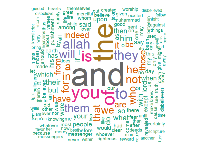
Figure 2.1: Wordcloud for Saheeh translation
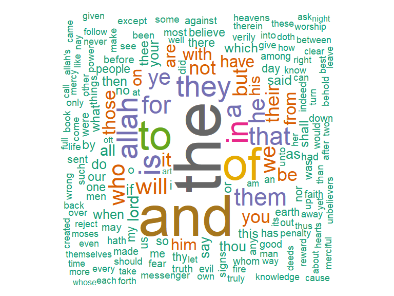
Figure 2.2: Wordcloud for Yusuf Ali translation
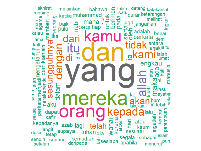
Figure 2.3: Wordcloud for Malay translation
For Saheeh, the wordcloud plot is in Figure 2.1; for Yusuf Ali, the wordcloud plot is in Figure 2.2; and for the Malay, the wordcloud plot is in Figure 2.3.
Obviously, the words such as “the” and “and” dominate the English versions, and “yang” and “dan” dominate the Malay version. These are “stopwords” in the languages, which we will deal with later. An English linguist may be able to discern the styles between Saheeh (which is American English) and Yusuf Ali (which is slightly older Engish) by observing the dominant usages of these stopwords.
Wordcloud tool is an easy and convenient way of visualizing word frequencies which we will be using throughout the book.
2.3 Analyzing word and document frequency
A central question in text mining and Natural Language Processing (NLP) is how to quantify what a document is all about. We can do this by looking at the words that make up the document. One measure of the importance of any word is its term frequency (tf), how frequently a word occurs in a document. There are words in a document that occur many times but may not be of any importance; in English, these are probably words like “the”, “is”, “of”, and so forth; in Malay, these are words like “dan” and “yang”. We might take the approach of adding words like these to a list of stopwords and removing them before analysis, but some of these words might be more important in some documents than others. A list of stopwords is not a very sophisticated approach for adjusting the term frequency for commonly used words.
Another approach is to look at a term’s inverse document frequency (idf), which decreases the weight for commonly used words and increases the weight for words that are not used very much in a collection of documents. We can use the term frequency to calculate its tf-idf (the two quantities multiplied together), a measure of the term’s frequency adjusted for how rarely it occurs in the whole text.
The tf-idf statistic is a measure of how important a word is to a document in a collection (or corpus) of documents, for example, to one novel in a collection of novels or one website in a collection of websites. In the case of the Quran, we can compare its properties between Surahs or Juz or Hizb.
The tf-idf is a rule-of-thumb or heuristic quantity. Simultaneously, it has proved useful in text mining and search engines. Its theoretical foundations are considered less than firm by information theory experts. The inverse document frequency for any given term is defined as:
\[idf(term) = \frac{ln[(number of documents)]}{(number of documents containing term)}\]
and tf-idf is defined as:
\[tfidf(term) = tf(term) * idf(term)\]
We can use tidy data principles to approach tf-idf analysis and use consistent, practical tools to quantify how various important terms are in a document that is part of a collection.
2.3.1 Term frequency in English Quran
We start by looking at the Surahs of the Quran and examine first term frequency, and then tf-idf. We can start just by using dplyr verbs such as group_by() and join(). We also calculate the total words in each Surah here, for later use.
surah_wordsESI <- quran_all %>%
  unnest_tokens(word, saheeh) %>%
  count(surah_title_en, word, sort = TRUE)
surah_wordsEYA <- quran_all %>%
  unnest_tokens(word, yusufali) %>%
  count(surah_title_en, word, sort = TRUE)
surah_wordsMAB <- quran_all %>%
  unnest_tokens(word, malay) %>%
  count(surah_title_en, word, sort = TRUE)

total_wordsESI <- surah_wordsESI %>%
  group_by(surah_title_en) %>% summarize(total = sum(n))
total_wordsEYA <- surah_wordsEYA %>%
  group_by(surah_title_en) %>% summarize(total = sum(n))
total_wordsMAB <- surah_wordsMAB %>%
  group_by(surah_title_en) %>% summarize(total = sum(n))

surah_wordsESI <- left_join(surah_wordsESI, total_wordsESI)
surah_wordsEYA <- left_join(surah_wordsEYA, total_wordsEYA)
surah_wordsMAB <- left_join(surah_wordsMAB, total_wordsMAB)
In the above codes, we create data.frame surah_wordsESI, surah_wordsEYA, and surah_wordsMAB, for each word-surah combination; n is the number of times that word is used in the Surah and total is the total words in the Surah. The usual suspects with the highest n are “the”, “and”, “to” (for English), and “dan”, “maka” (for Malay).
In the following figures, we look at the distribution of \(\frac{n}{total}\) for surahs grouped by the Surahs’ length. The term frequency is the number of times a word appears in a surah divided by the total number of terms (words) in that Surah.
We start first with the short Surahs at the end of Al-Quran, then to the medium length Surahs, and finally to the long Surahs (similar to when we normally start to learn Al-Quran, starting to learn reading Al-Quran by learning the shorter ones first, followed by the longer ones).
last6_surahs = c("An-Naas", "Al-Falaq", "Al-Ikhlaas", "Al-Masad","An-Nasr", "Al-Kaafiroon")
hamim_surahs = c("Ghafir", "Fussilat", "Ash-Shura", "Az-Zukhruf", "Ad-Dukhaan", "Al-Jaathiya")
long_surahs = c("Al-Baqara", "Aal-i-Imraan", "An-Nisaa", "Al-Maaida","Al-An'aam", "Al-A'raaf")
tf_plotter = function(df,surah_group,title_label,x_lim){
df %>%
filter(surah_title_en %in% surah_group) %>%
ggplot(aes(n/total, fill = surah_title_en)) +
geom_histogram(show.legend = FALSE) +
xlim(NA,x_lim) +
facet_wrap(~surah_title_en, ncol = 2, scales = "free_y") +
labs(title = title_label,
x = "Term Frequency",
y = NULL)+
theme(plot.title = element_text(size=12),
# panel.border = element_rect(colour = "black", fill=NA),
strip.background = element_rect(color = "black"),
plot.background = element_rect(color = "black"))
}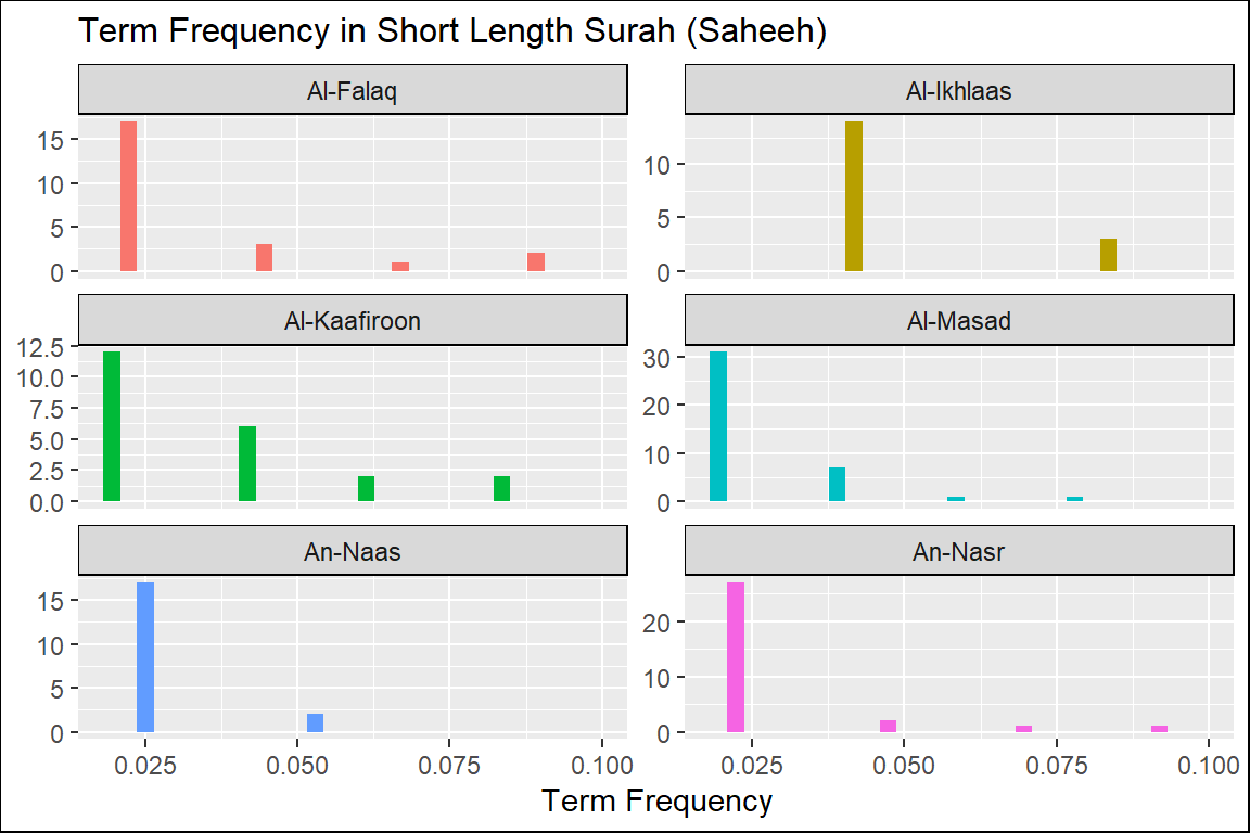
Figure 2.4: Short Surahs term frequency in Saheeh
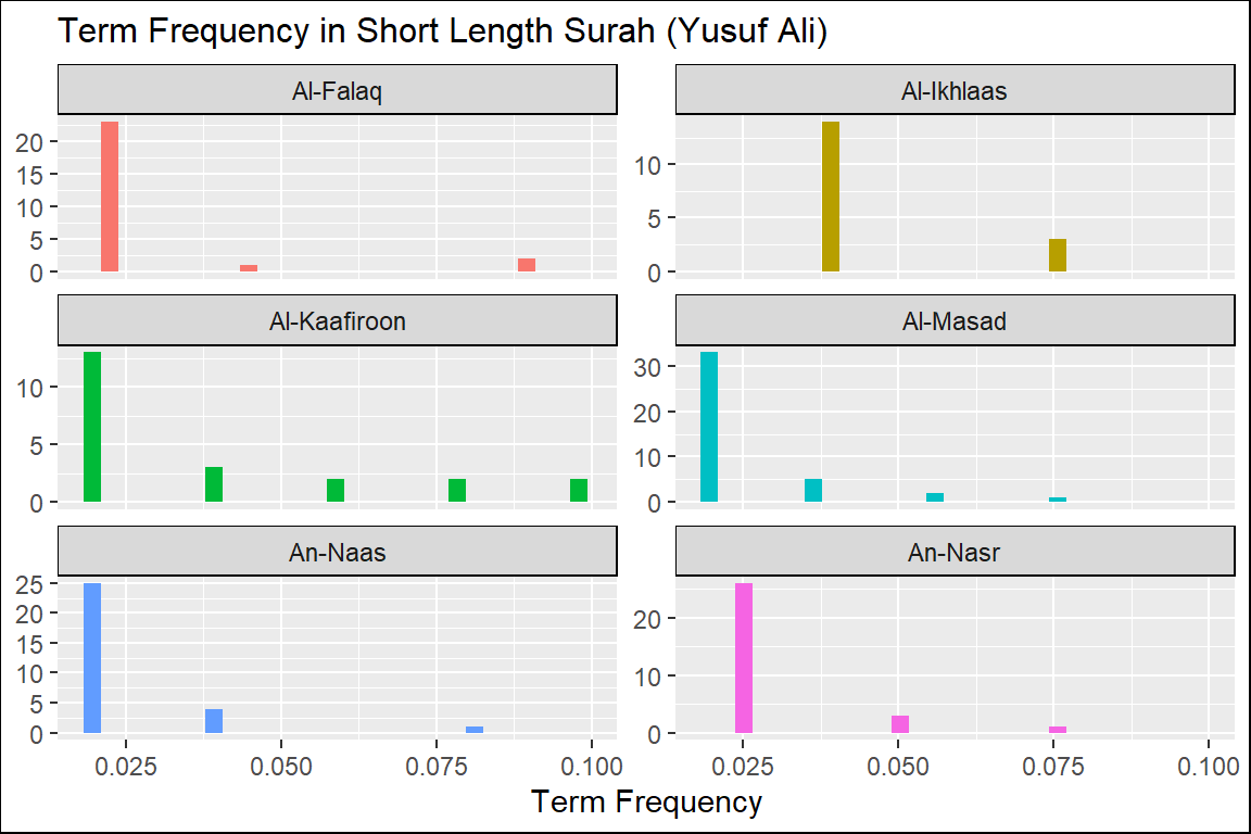
Figure 2.5: Short Surahs term frequency in Yusuf Ali
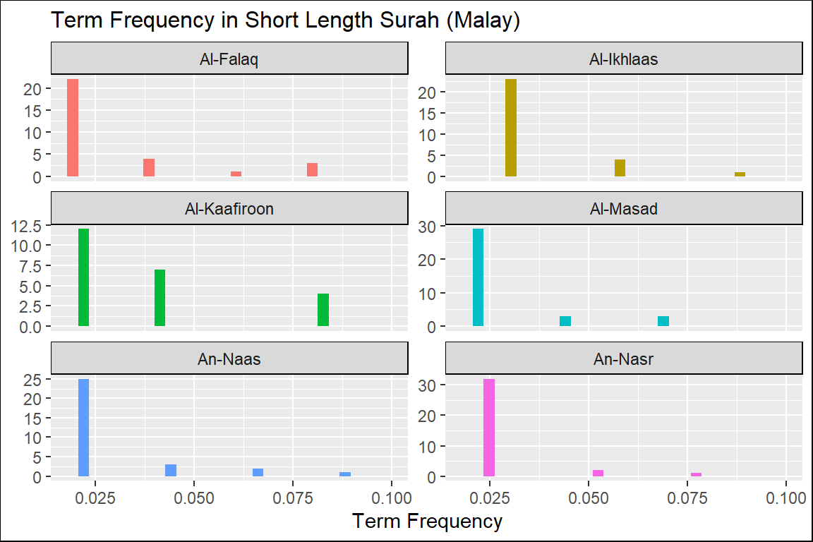
Figure 2.6: Short Surahs term frequency in Malay
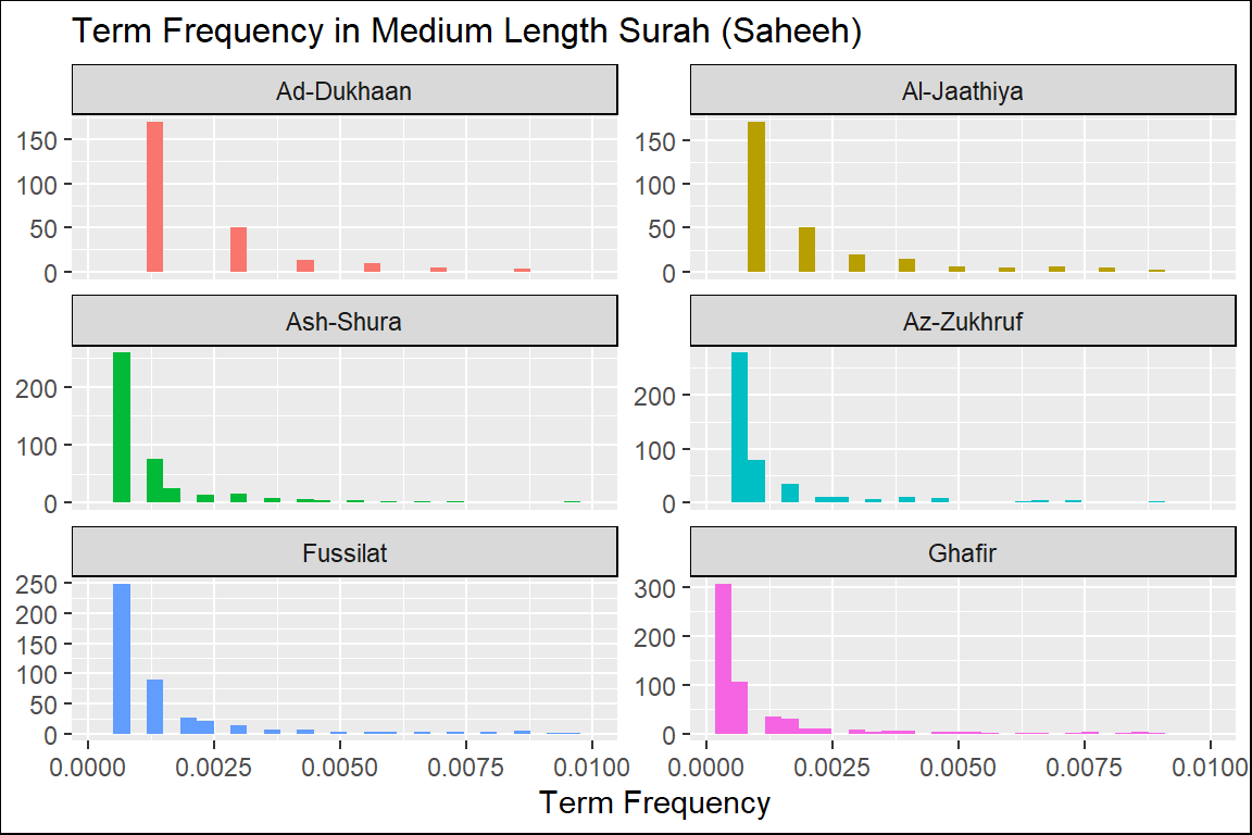
Figure 2.7: Hamim Surahs term frequency in Saheeh
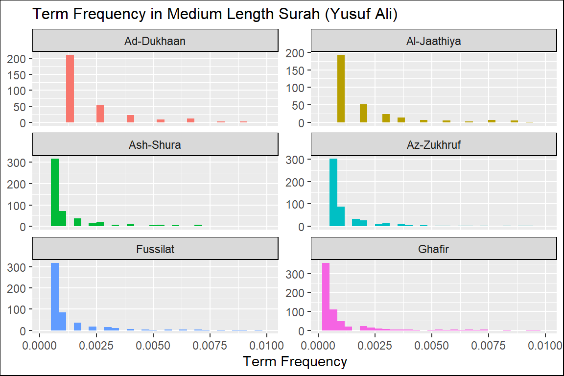
Figure 2.8: Hamim Surahs term frequency in Yusuf Ali
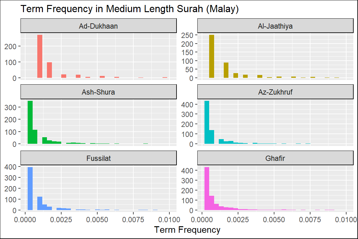
Figure 2.9: Hamim Surahs term frequency in Malay
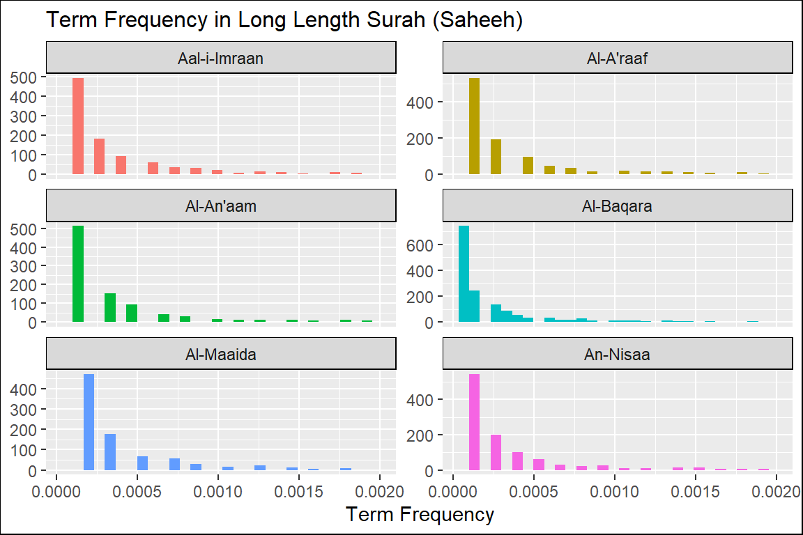
Figure 2.10: Long Surahs term frequency in Saheeh
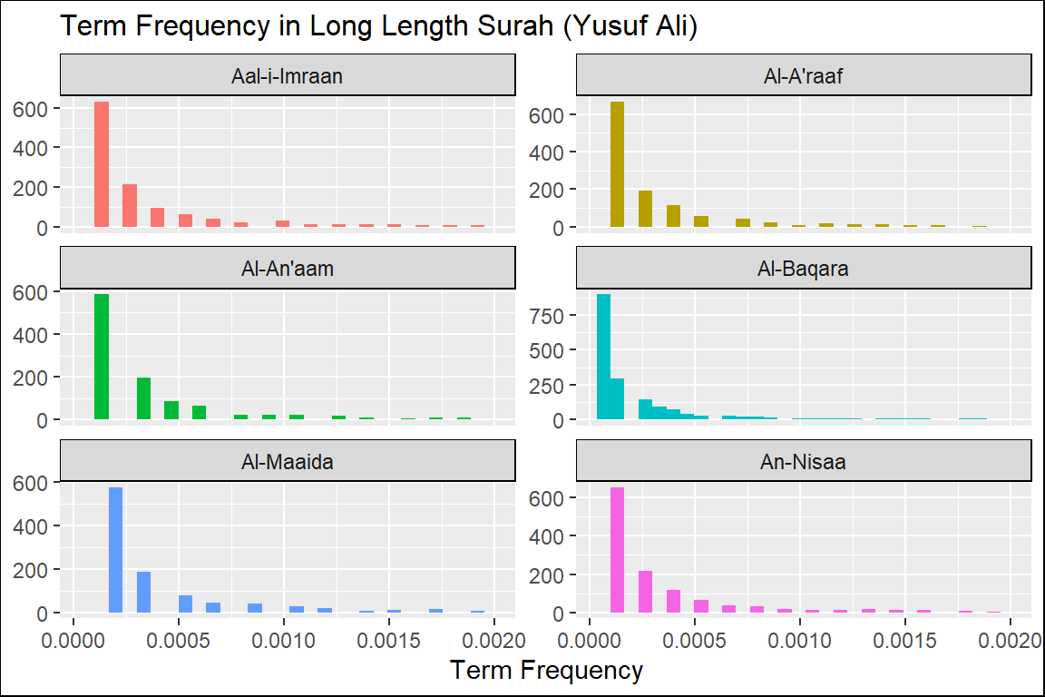
Figure 2.11: Long Surahs term frequency in Yusuf Ali
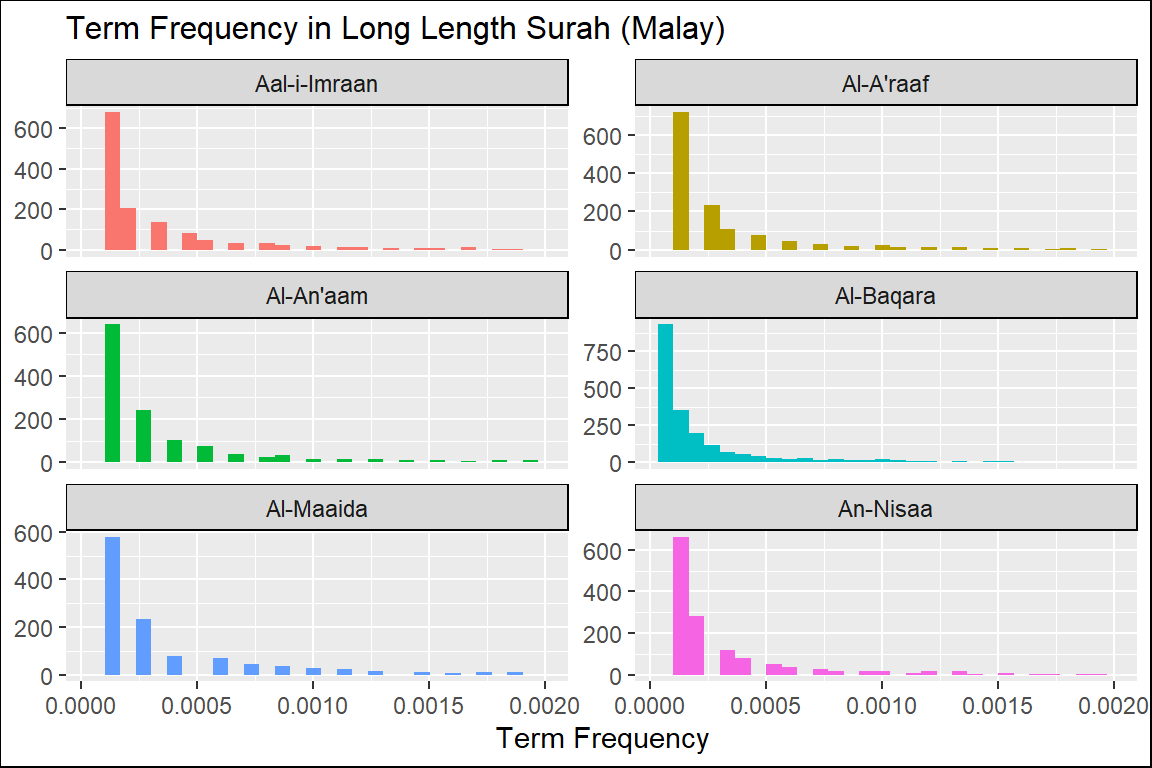
Figure 2.12: Long Surahs term frequency in Malay
From these plots of “term frequency” starting with the short Surahs (Figure 2.4, Figure 2.5, and Figure 2.6), followed by the medium Surahs (Figure 2.7, Figure 2.8, and Figure 2.9), and the long Surahs (Figure 2.10, Figure 2.11, and Figure 2.12), there are many insights and lessons about the language of the translation of Al-Quran.
For example, we can observe that the term frequencies for all the translations showed “scale-invariant properties” to the language and terminologies used to translate the Quran. Scale-invariant refers to the fact that despite different filters used (a translation is a filtering method), the resulting outputs exhibit similar properties; this is an important observation about the structure of the original texts of the Quran in Arabic. An example of scale-invariancy is sign languages for deft and mute people - whereby it is known to be language-specific independent. Are the translated messages in the Quran, aside from the original text, language-independent?
There are many more analyses open to the researchers by studying the various structures and properties of the word frequencies in the original texts against the translated texts of Al-Quran. We leave this for future work and research.
To have a broader view of the observations made, let us look at the plot for the percentages of unique words (tokens) against the total number of words (tokens) within each Surah for all the translations.
library(reshape2)
EQT_total_toks = data.frame("Surah" = 1:nrow(ESI_total_toks),
                            "Saheeh" = ESI_total_toks$percentage,
                            "YusufAli" = EYA_total_toks$percentage,
                            "Malay" = MAB_total_toks$percentage)
EQT_total_toks_melt = melt(EQT_total_toks,
                           id.vars = "Surah",
                           variable.name = "Translation",
                           value.name = "Percentage")
EQT_total_toks_melt %>% ggplot() +
                            geom_point(aes(x = Surah,
                                           y = Percentage,
                                           shape = Translation,
                                           color = Translation))  +
                            labs(x = "Surah number",
                                 y = "Percentage",
                                 title = "Percentage of Unique Words in Surah") +
  scale_y_continuous(labels = scales::percent)+
  theme(panel.border = element_rect(colour = "black", fill=NA))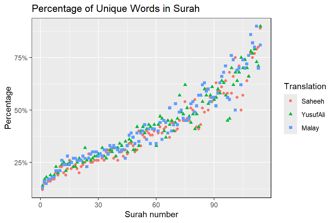
Figure 2.13: Percentage of unique words in the Surahs
The percentage of “unique words” over “total words” is a measure of the lexical variety within a sub-set of texts (i.e., Surah). The plot in Figure 2.13 shows that the lexical variety in the shorter Surahs varies more than the longer Surahs. It is quite rare in any regular text collection that a shorter group of sentences (such as chapters) display more outstanding lexical varieties. The case is different here.
We can see that while all the translations differ in the languages and styles, the lexical varieties in the shorter Surahs are consistently higher. An implication of this is that, while many of the Surahs in Al-Quran may be short, they convey distinctively different messages.
2.3.2 The bind_tf_idf function
The concept of tf-idf is to measure the degree of importance of words within the content of each group of texts, such as a Surah, by decreasing the weight for commonly used words and increasing the weight for words used less. We want to detect commonly occurring words, but not too common. In general textual analysis, these words represent a topic of interest, the headlines, the themes, or a subject that stands above other surrounding texts. It is an essential tool for understanding text structures and uncovering the messages in texts.
The idf’s and thus tf-idf’s for the highly used words, such as the word “the”, is zero. These are all words that appear in all 114 Quran Surahs, so the idf term (which will then be the natural log of 1) is zero. It is also very low (near zero) for words that occur in many documents (i.e., Surahs) in a corpus. Furthermore, the inverse document frequency will be higher for words that occur in fewer of the sub-set of documents (i.e., Surahs) in the corpus. Therefore, words of which idf’s and tf-idf’s are near zero, and yet not near enough are what we are looking for.
The bind_tf_idf function in the tidytext package takes a tidytext dataset as input with one row per token (term), per document. One column (a column named word) contains the terms/tokens, one column contains the documents (Surah in this case), and the last necessary column contains the counts, how many times each document contains each term (n in this example).
First, let us plot the tf-idf for all three translations and make some observations.
surah_wordsESI <- surah_wordsESI %>%
  bind_tf_idf(word, surah_title_en, n)
surah_wordsEYA <- surah_wordsEYA %>%
  bind_tf_idf(word, surah_title_en, n)
surah_wordsMAB <- surah_wordsMAB %>%
  bind_tf_idf(word, surah_title_en, n)
ESI_tf_idf = surah_wordsESI %>%
                select(-total) %>% arrange(desc(tf_idf))
EYA_tf_idf = surah_wordsEYA %>%
                select(-total) %>% arrange(desc(tf_idf))
MAB_tf_idf = surah_wordsMAB %>%
                select(-total) %>% arrange(desc(tf_idf))

tfidf_plotter = function(df_plot,title_label,color){
                ggplot() +
                geom_point(aes(x = 1:length(df_plot$tf_idf),
                       y = log(df_plot$tf_idf)), color = "red",
                       size = 0.05) +
                labs(title = title_label, x = "n", y = "tf_idf")+
                theme(panel.border = element_rect(colour = "black", fill=NA),
                      axis.text.x = element_text(angle = 45,vjust = 0.5))
  }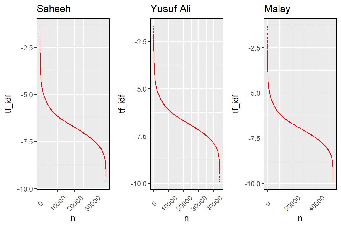
Figure 2.14: tf-idf for the translations
We can see from Figure 2.14, the structure for all the translations looks similar; the differences are due to the number of words in each translation. What is striking is despite all the variety of words and language used, the structure of tf_idf is almost perfectly the same (and in fact, they are the same if we normalize the scale by the number of total words). It is clear that there are some words which used rarely (the curves on the left side, with high tf_idf), the numbers of which are not that many, and there are words that are used extremely frequently (the curves on the right side, with low tf_idf), the numbers of which are not that many; and the rest of the words are used moderately (in between).
Let us look at a visualization for these high tf-idf words. These are shown in Figure 2.15, Figure 2.16, Figure 2.17, Figure 2.18, Figure 2.19, Figure 2.20, Figure 2.21, Figure 2.22, and Figure 2.23.
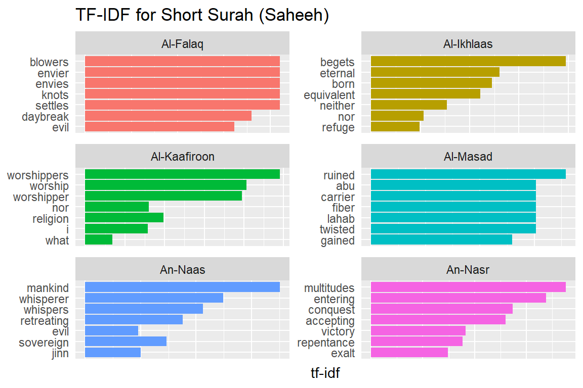
Figure 2.15: Short Surahs tf-idf for Saheeh
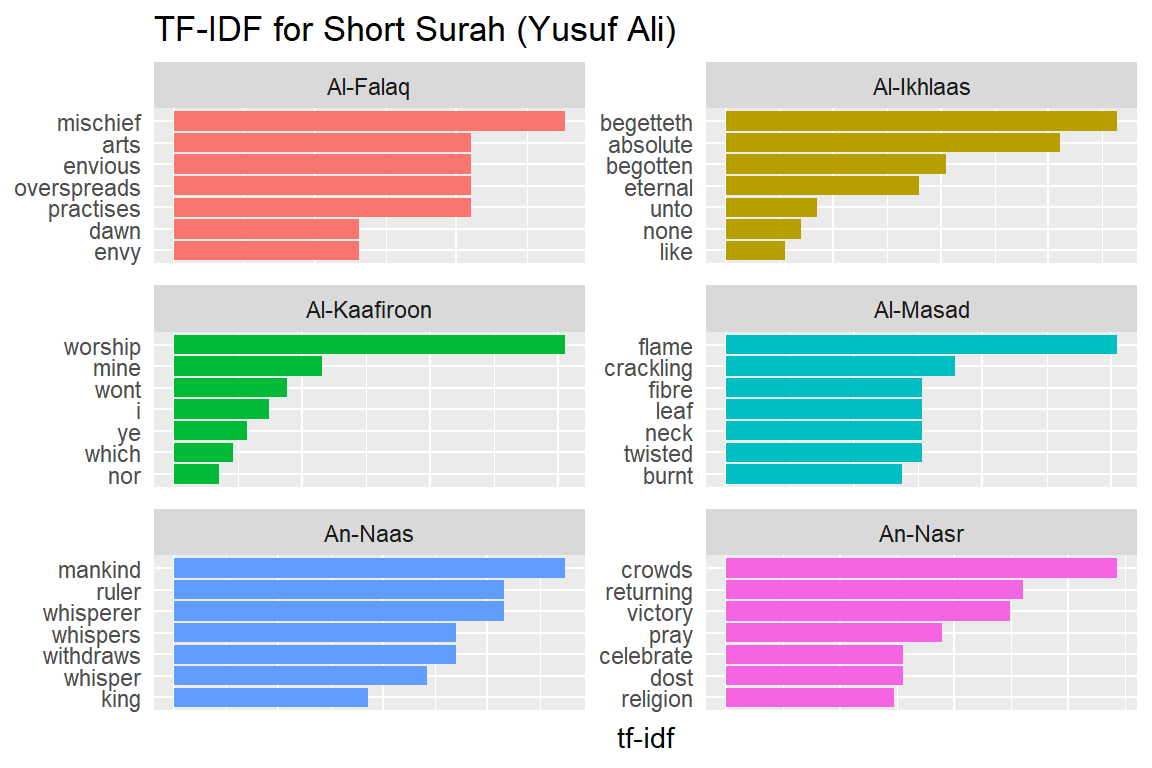
Figure 2.16: Short Surahs tf-idf for Yusuf Ali
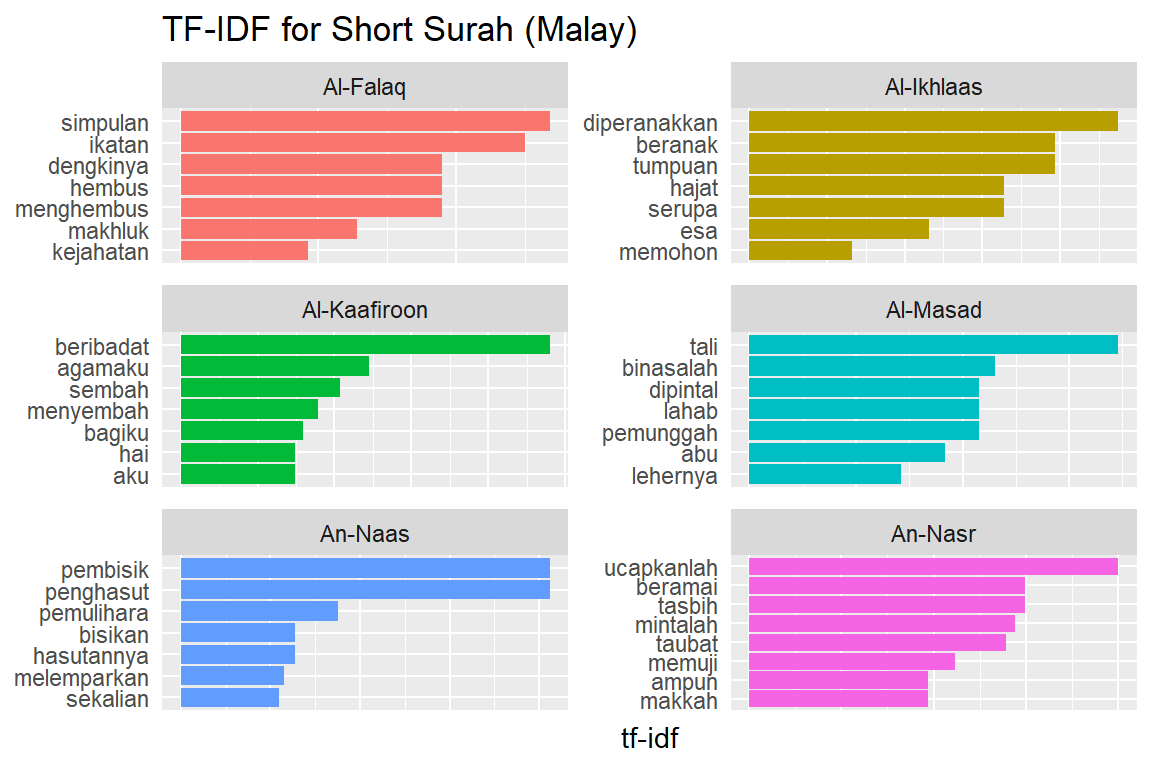
Figure 2.17: Short Surahs tf-idf for Malay
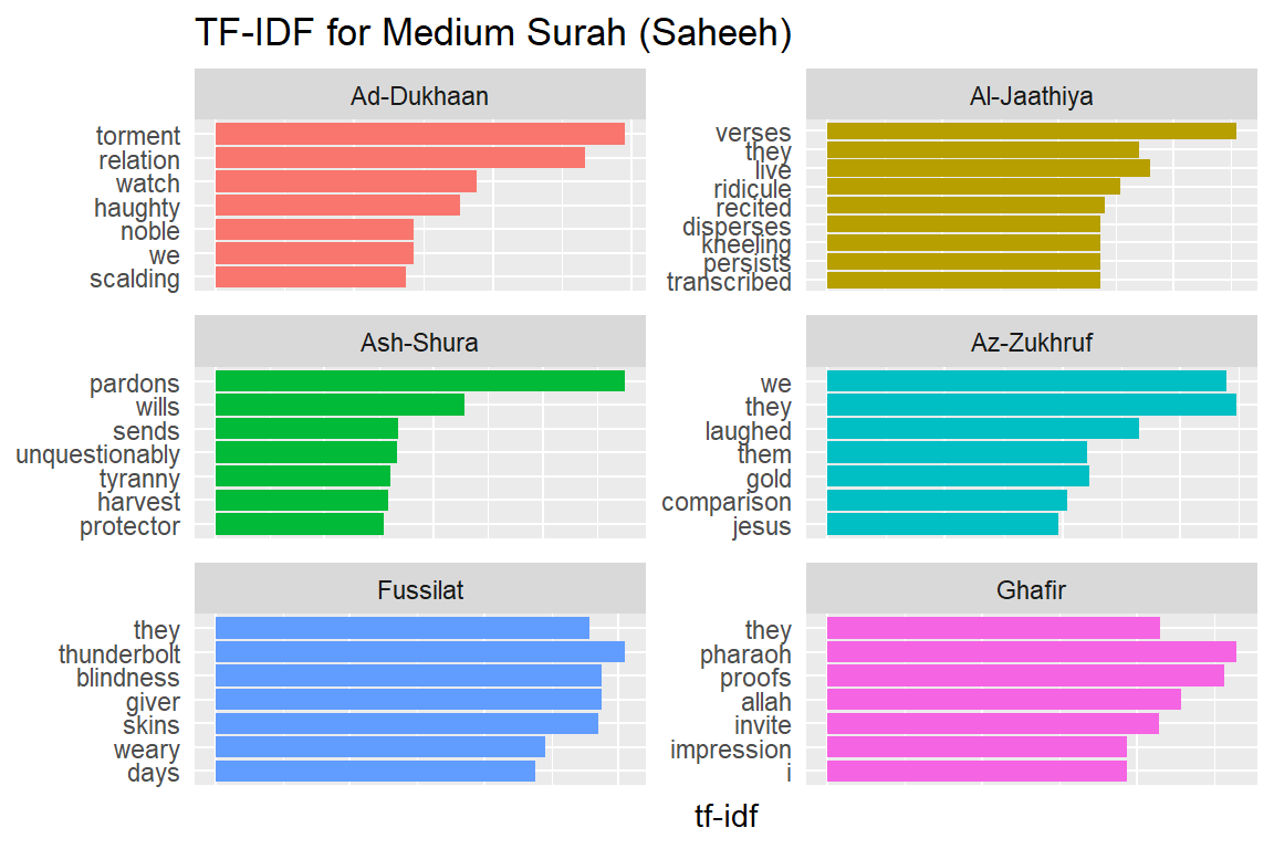
Figure 2.18: Medium Surahs tf-idf for Saheeh
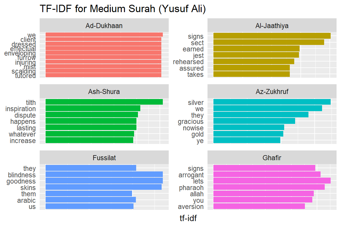
Figure 2.19: Medium Surahs tf-idf for Yusuf Ali
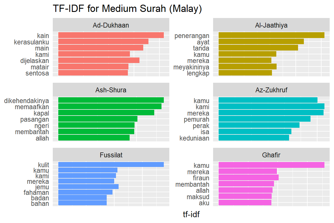
Figure 2.20: Medium Surahs tf-idf for Malay
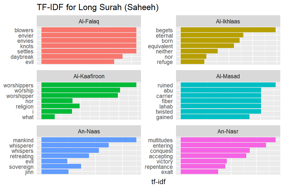
Figure 2.21: Long Surahs tf-idf for Saheeh
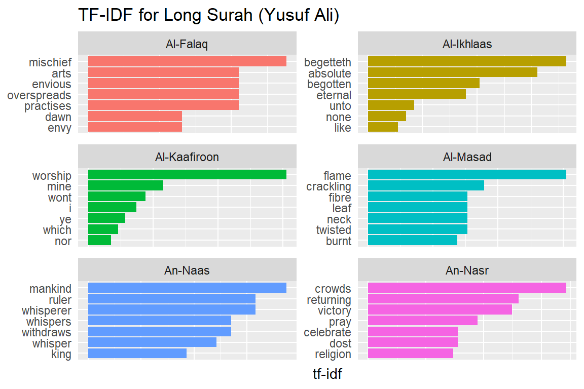
Figure 2.22: Long Surahs tf-idf for Yusuf Ali

Figure 2.23: Long Surahs tf-idf for Malay
As measured by the tf-idf, these words are the most important to each Surah, and most readers would likely agree. It identifies words that are important to one document within a collection of documents. Furthermore, we can see that Saheeh’s translation used different words than Yusuf Ali; this is obvious in the top tf_idf terms where they differ significantly.
The shape of the tf-idf curves has many similarities between the translations; the terms (or words) they use are not the same, while clearly, they are only translations of the same Arabic verses. These observations raise a question: do different translation methods bring different meanings to the readers? Will this alter the message contained in the original texts?
2.4 Zipf’s law
Zipf’s law states that the frequency of a word’s appearance is inversely proportional to the rank of its frequency for a given corpus. In general, Zipf’s law states that the frequency distributions of words in a corpus follow a Power Law behavior (Zipf 1949). The words such as “allah” in the translations, for which the term frequency is high, are inversely related to its rank, which is low. A Power Law distribution from a statistical perspective is a distribution with both a fat tail and a long tail simultaneously. Power Law has many implications for statistical testing and scale-free network behaviors (a subject beyond the current discussion).
Here we present the Zipf’s plots for the translations, indicating whether they follow Zipf’s law (and hence power-law) and test the translations’ similarities.
freq_by_rank_ESI <- surah_wordsESI %>%
  group_by(surah_title_en) %>%
  mutate(rank = row_number(),
         `term frequency` = n/total) %>%
  ungroup()
freq_by_rank_EYA <- surah_wordsEYA %>%
  group_by(surah_title_en) %>%
  mutate(rank = row_number(),
         `term frequency` = n/total) %>%
  ungroup()
freq_by_rank_MAB <- surah_wordsMAB %>%
  group_by(surah_title_en) %>%
  mutate(rank = row_number(),
         `term frequency` = n/total) %>%
  ungroup()

zipf_plotter = function(freq_rank_df,title_label){
  freq_rank_df %>%
  ggplot(aes(rank, `term frequency`, color = surah_title_en)) +
  geom_line(size = 0.5, alpha = 0.8, show.legend = FALSE) +
  geom_abline(intercept = -0.62, slope = -1.1,
              color = "black", linetype = 2) +
  scale_x_log10() +
  scale_y_log10() +
  labs(title = title_label,
       x = "Log of Rank",
       y = "Log of Term Frequency")+
    theme(panel.border = element_rect(colour = "black", fill=NA))
}
p1 = zipf_plotter(freq_by_rank_ESI,"Saheeh")
p2 = zipf_plotter(freq_by_rank_EYA,"Yusuf Ali")
p3 = zipf_plotter(freq_by_rank_MAB,"Malay")
cowplot::plot_grid(p1,p2,p3, nrow = 1)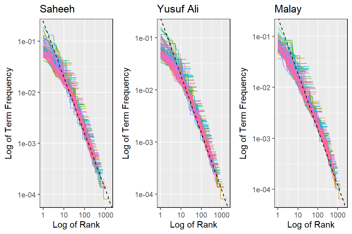
Figure 2.24: Zipf’s plot
Note that the plot in Figure 2.24 is on a log-log scale (for testing Power Law), whereby if the lines are close to the inverse 45-degree line, then the law holds. We can see that all plots indicate a broad indication of adherence to Zipf’s law. Based on this, we can conclude that all translations explain the same subject in broad terms, despite earlier indications of differences of styles. A visual test of the power-law is insufficient, and a full and proper test is required to prove this point, which is beyond the current scope of this book.
2.5 Words of high occurrence and stopwords
From the wordcloud plots in Figure 2.1, Figure 2.2, and Figure 2.3, we can see consistently the connecting terms emerged as high frequency terms for all versions of translation. The question is, how do we treat some words which occur in high frequencies, such as these connecting words, and at the same time, having low inverse ranking? Should these words remain in the texts or removed for the (statistical) analysis since their roles are more as word connectors rather than carrying any meaning? Is the decision to take out these words justified?
Most analyses of texts in English will take the option of removing these stopwords. While maybe acceptable in most circumstances, such an approach is not as straightforward when applied to Al-Quran translations. In the coming chapters, we will revisit the subject again. Let us redo Zipf’s plot with all the stopwords removed and see what the removal of stopwords means.
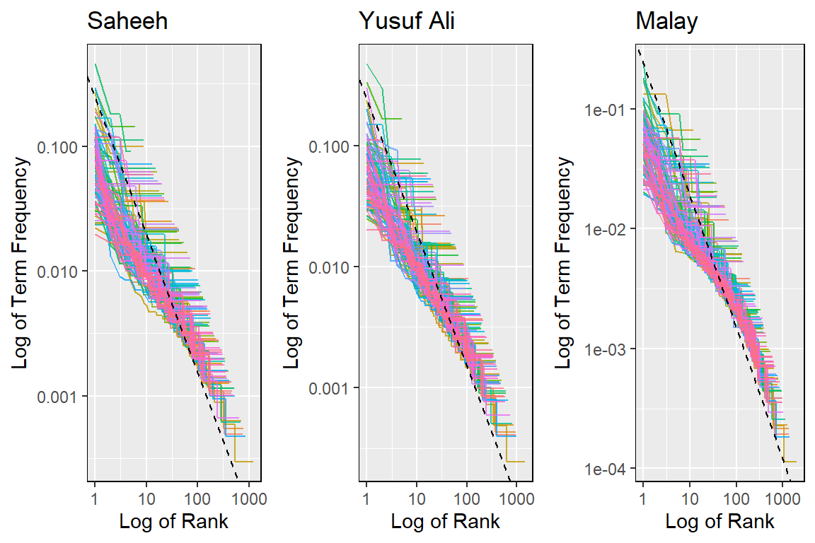
Figure 2.25: Zipf’s plot without stopwords
From the plots in Figure 2.25, compared to the previous Zipf’s plot in Figure 2.21, we can observe significant changes when we removed the stopwords. Putting the three translations together indicates that while removing the stopwords changes the texts’ structure, it might not change the texts’ meaning since the translations demonstrate similarities after their removal. In other words, the translations’ texts are robust to changes due to these connector words. This is the nature of the English language as explained by Zipf (Zipf 1949), and probably it is the same for the Malay language. However, are we sure that the meanings are retained? This must be proven beyond doubt for it to be conclusively accepted.
We caution the readers that we have been rather casual in some of the claims without rigorously providing statistical tests or proofs. Instead, we rely only on the visualizations provided and let the “data illustrate itself”. Our purpose is to highlight various indications for future work and research and at the same time, allow readers with no statistical background, to understand the concepts and approach. The need for a full and proper test of the hypothesis as indicated above is one example case of precaution required before concluding.
2.6 Words of rare occurrence
Another method of analysis in word statistical analysis for corpus linguistics is to study hapax legomenon (singular) or hapax legomena (plural). It is about words that occur only once or extremely infrequently within the corpus. Examples of this in Al Quran are: “harut”, “marut”, and “zanjabil”.38 Studying hapax legomena helps us in understanding how different authors’ (in our case here, translators) approach the usage of dictionary and vocabulary.
The subject of hapax legomena in linguistics requires a much more in-depth analysis, which we do not intend to perform in this book.39 Here we will do a simple explanatory analysis demonstrating the uses of hapax legomena in text analysis.
The table below describes a summary of the number of (words) tokens and unique tokens (words). Please note the numbers for the Al-Quran Arabic for comparison.
| Item | Al-Quran40 | Saheeh | Yusuf Ali | Malay |
|---|---|---|---|---|
| Total number of tokens | 77,430 | 158,065 | 167,859 | 204,784 |
| Total number of unique tokens | 18,994 | 5,251 | 6,365 | 7,156 |
Unique tokens are similar to vocabulary in some sense. It is the library of words used in the corpus. Comparing English and Malay versus Arabic, indicates clearly that the structure of language is starkly different. Arabic consists of much lower tokens (less verbose) and yet higher unique tokens (larger library), while Saheeh and Yusuf Ali are the opposite (more verbose, smaller library); and Malay on the other hand needs much more words (much more verbose) with smaller library than Arabic, and larger than the English corpora. (The Malay translation often includes explanations in the main text. That may explain the larger number of tokens used compared to the number of unique tokens.)
As we have described before, in the corpora, few words occur in high frequencies, and few words occur in very low frequencies at both extremes. We will plot the statistical density of the distribution (in log scale) of the term frequencies in both translations to observe this phenomenon.
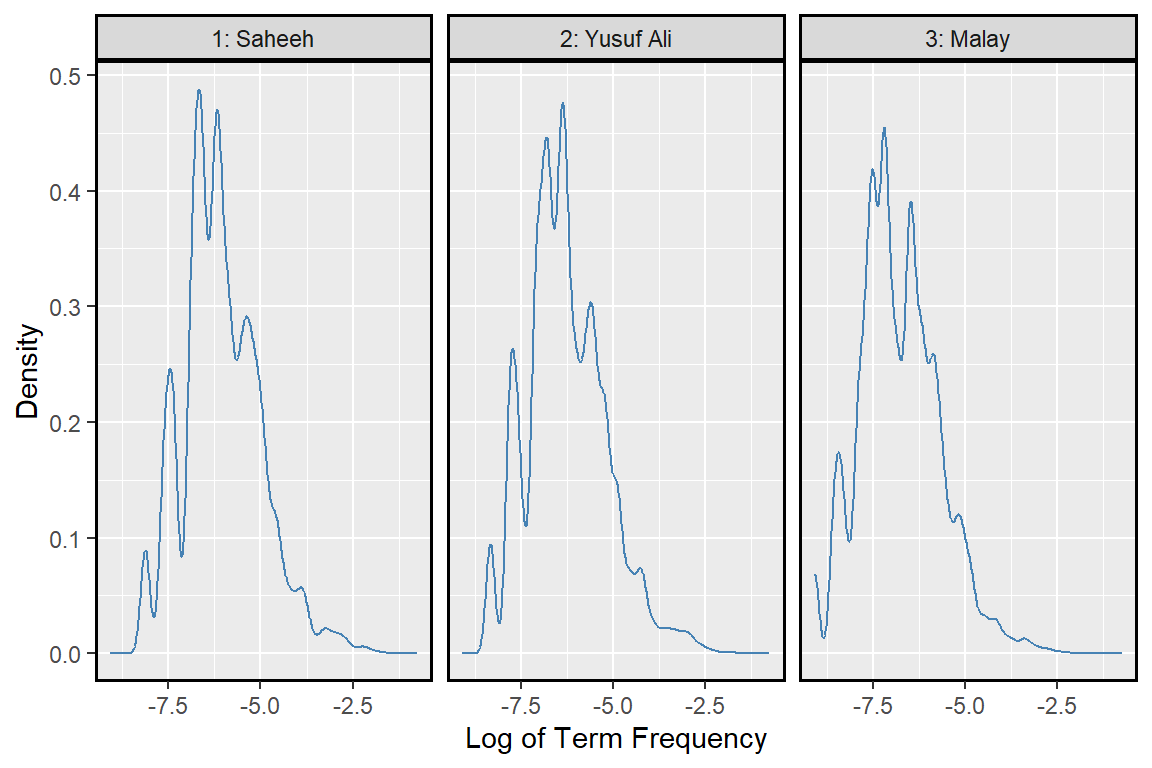
Figure 2.26: Density plot of term frequency
The term frequencies (using a log scale for visualization) for both translations in Figure 2.26 show striking similarities, despite the style difference. On the left are the terms which occur infrequently, and as we add more terms to the vocabulary (as we move to the right), the density curve peaked at few distinct modes until it flattens out to the right as we bring into the vocabulary words frequently used. If we check what are the words on the left, examples would be “harut”, “marut”, “iram” (which are unique names), and in the middle are words like “food”, “eat”, “makan” (which are common words), and finally in the far right are words like “with”, “the”, “yang” (which are the stopwords).
An important observation is why the density curves have multiple “peaks”; there are two lower peaks on the left, and a few peaks in the middle, and a fat tail to the right. Is this structure common in any English corpus or Malay corpus? Or this is true only in the case of translations of Al-Quran. Comparisons between the corpora under study with other common corpora are required to confirm this phenomenon.41
The subject of vocabulary and rare word usage is essential and extensive by itself. In particular, term frequencies analysis of rare occurrence words may yield insights of its own, which revolves around why and how hapax legomena exists in communications and vocabulary development in languages. As a case in point, usage of words with multiple synonyms, such as “abrogate” versus “evade”; which one is a more appropriate choice for a given original Arabic word? Comparing these words against its original Arabic word would be interesting since the Arabic may carry its distinctive meaning, while in contrast, the English word equivalent may carry its content or context.
We would like to show some of the types of analysis of rare words which may carry significant meanings, such as the word “trustworthy” and “trust”. “Trustworthy” occurs only 13 times in Saheeh and 3 times in Yusuf Ali, while “trust” occurs only 3 times in Saheeh and many times in Yusuf Ali. The exact occurrences are shown below:
## # A tibble: 8 × 6
##   surah_title_en word            n total  rank `term frequency`
##   <chr>          <chr>       <int> <int> <int>            <dbl>
## 1 Ash-Shu'araa   trustworthy     6   729    20         0.00823
## 2 Ad-Dukhaan     trustworthy     1   209   141         0.00478
## 3 Al-A'raaf      trustworthy     1  1838   764         0.000544
## 4 Al-Baqara      trustworthy     1  3401  1166         0.000294
## 5 Al-Qasas       trustworthy     1   753   388         0.00133
## 6 An-Naml        trustworthy     1   631   359         0.00158
## 7 At-Takwir      trustworthy     1    79    68         0.0127
## 8 Luqman trustworthy 1 318 195 0.00314## # A tibble: 3 × 6
## surah_title_en word n total rank `term frequency`
## <chr> <chr> <int> <int> <int> <dbl>
## 1 Al-A'raaf trustworthy 1 2326 925 0.000430
## 2 Al-Baqara trustworthy 1 4120 1383 0.000243
## 3 Luqman trustworthy 1 384 233 0.00260## # A tibble: 3 × 6
## surah_title_en word n total rank `term frequency`
## <chr> <chr> <int> <int> <int> <dbl>
## 1 Aal-i-Imraan trust 1 2025 737 0.000494
## 2 Al-Ahzaab trust 1 793 387 0.00126
## 3 Al-Baqara trust 1 3401 1165 0.000294## # A tibble: 27 × 6
## surah_title_en word n total rank `term frequency`
## <chr> <chr> <int> <int> <int> <dbl>
## 1 Ash-Shu'araa trust 6 929 26 0.00646
## 2 Aal-i-Imraan trust 5 2448 88 0.00204
## 3 Yusuf trust 5 1195 36 0.00418
## 4 Al-Anfaal trust 4 893 36 0.00448
## 5 Al-Baqara trust 4 4120 233 0.000971
## 6 Ibrahim trust 4 639 21 0.00626
## 7 Al-Ahzaab trust 3 928 62 0.00323
## 8 Hud trust 3 1314 108 0.00228
## 9 Yunus trust 3 1171 97 0.00256
## 10 Al-Maaida trust 2 1995 301 0.00100
## # ℹ 17 more rowsOnly three occurrences of “trustworthy”, in Surah Al-A’raaf, Al-Baqara, and Luqman, coincide in both translations. In Saheeh’s Surah Ash-Shu’araa, it occurs six times and is not present in Yusuf Ali. Further checks reveal that in Yusuf Ali’s Surah Ash-Shu’araa, instead of Saheeh’s “trustworthy”, “worthy of trust” is used in its place. Why Yusuf Ali prefers the word “trust” more than Saheeh is a subject worthy of understanding by itself. Furthermore, as we can see from the outputs, the tf-idf measures reveal the words’ positions within the Surah and the corpus, which is an indicator of its own understanding.
We showed here many dimensions of analysis using words, word frequencies, inverse frequencies, word positions within a sub-set of texts (i.e., Surahs), and the whole corpus, across corpora. These analyses are rich in understanding and knowledge of linguistics, meanings, and contexts. We also showed the intricacies involved in word selection for translations like the case for “trust”, “trustworthy”, and “worthy of trust”.
2.7 Words with medium occurrence
What do words of non-high occurrence and non-rare occurrence, hence medium occurrence, represent? For once we know that these words represent the largest part of the vocabulary library for each corpus.
Let us take Saheeh as our example. The highest rank is “allah” (rank = 1), and among the lowest rank is “wombs” (rank = 1199). Let us check what are the words in the middle rank, rank around 600.
We can see words, such as “oaths”, which describe an action, occurs 13 times in the Saheeh corpus. Similarly the name of the Prophet Noah, which occurs 28 times; which case is different since the word is a special name. Another word, such as “masjid” which generally means the mosque, occurs 9 times. We can see that these middle-frequency words are non-trivial since they do hold a special purpose within a certain context and meaning; for example, we have a very strong action, which is an oath, a special name, which is the Prophet Noah, and a special place, a Mosque.
Words of mid-frequency occurrence become very important when we need to go deeper into the context and meaning of words, sentences, groups of sentences (such as Surahs) - a subject that we will revisit in later chapters.
2.8 Summary
While seemingly simple, statistical word analysis yields many insights into issues relating to a corpus of texts. In this chapter, we have shown examples of how the analysis is useful for many linguistic studies of Al-Quran translations. We also compared different translations of the English language (Saheeh and Yusuf Ali) and different languages (English and Malay).
Analysis using term frequency (tf) and inverse document frequency (idf) allows us to find word characteristics for one document within a collection of documents. Exploring term frequency on its own can give us insight into how language is used in a collection of natural language and give us tools to reason about term frequency. The proper noun “Allah” ranks very high on almost all the statistics of the English Quran which confirms that “Allah” is the central and most important subject matter of the Quran, a topic that one of the authors will cover in an upcoming book (Alsuwaidan and Hussin 2021).
Statistical analysis of words from the Quran is a good and “easy” start to Quran Analytics. It is general and robust, requires no or little manual effort, and is “surprisingly” powerful. As we have indicated in this chapter’s various suggestions, the subject requires further research. Among the issues raised is about translations of Al Quran into another language, such as the English and Malay language (as the case here), which has its structural dependencies. Will the usage of different structure results in a difference in meaning and understanding? Is there any better way to detect and compare different writing styles to ensure or reflect accurate meaning to the readers? How does the usage of infrequent words add to the vocabulary richness of the texts? The words statistical analysis is a starting point to answer these types of questions and many other questions a researcher of Al-Quran may explore.
We leave this chapter and many of the issues raised for future research works. The following is an incomprehensive list of what’s possible:
Statistical NLP, which is based on word frequencies, has a lot to offer. Within a language, across languages, for purposes of translations between languages, are open examples. Al-Quran, a sacred text for the Muslims, must be translated with care. The various authors have done all existing translations based on their styles and understanding of both the original texts (in Arabic) and the language of translation. There is a need to revisit this subject using NLP tools to provide a reflective meaning suitable for the current time.
Word frequency analysis is among the simplest tool available yet provides many insightful understandings of language. We also covered Zipf’s law, scale-free, power-law distributions of word frequencies. We showed how words of high occurrence, which are stopwords and words of importance, reveal many insights about the language and the messages in texts; while words of extremely low occurrence, hapax legomena, direct towards vocabulary usages and special meanings. All of these mentioned items can be extended as a research subject by themselves.
An example of classical work in Arabic for Al-Quran word-by-word references is Al-Mu’jam Al-Mufahras Li Alfaz Al-Quran Al-Kareem by Muhammad Fu’ad Abdul-Baqi (Abdul-Baqi (1945)). If the works in Al-Mu’jam are converted to tokens’ data structures as we have done for the English or non-Arabic texts, cross-referencing can be quickly done. Using this tool, any Quranic scholar can check the accuracy or appropriateness of the Quranic translations with ease. It is among the examples of why we need the tools of NLP for Quran Analytics.
The simplest tools of data science, namely simple statistical tests, have not been explored to their full potentials. The power of data visualizations using programming languages such as R, as we have done here, is enormous.
The room to improve and expand on “word frequency analysis” is tremendous. We are just at its beginning stage.
2.9 Further readings
Abdul-Baqi, M. F. Al-Mu’jam Al-Mufahras Li Alfaz Al-Quran Al-Kareem. Dar Ahi’a Al-Tirath Al-Arabi, Beirut, Lebanon, 1945. (Abdul-Baqi 1945)
Alsuwaidan, T. and Hussin, A. Islam Simplified: A Holistic View of the Quran. To be published manuscript, 2021 (Alsuwaidan and Hussin 2021)
Zipf, G. K. Human Behavior and the Principle of Least Effort. Addison-Wesley, New York, New York, 1949. (Zipf 1949)
tidytext package in R. (Queiroz et al. 2020)
ggplot2 package in R. (Wickham et al. 2020)
quRan package in R. (Heiss 2018)
Tidy text mining website: https://www.tidytextmining.com/tidytext.html
References
This may indicate that in general, the Malay language is more verbose than the English language or the author may have included some commentaries within the text of the verse, usually in parenthesis.↩︎
https://en.wikipedia.org/wiki/Hapax_legomenon#Arabic_examples↩︎
In R, there are a few packages which are useful for the analysis, a notable one is qdap (http://trinker.github.io/qdap/vignettes/qdap_vignette.html) which stands for “Quantitative Discourse Analysis Package”.↩︎
We will leave this subject as a research question.↩︎