4 Word Collocations
The word is among the most elementary units of language. It forms the vocabulary, is part of the grammatical structures, builds the semantics of a sentence, and provides many contexts of usage. Among the important tools developed in NLP is to model the relationships between words, in a sentence, in a corpus, and across corpora of text collection. Sentences or speeches are organized as sequences of words, upon which the concept of word relations is built.
In this chapter, we will cover the broad ideas on the role of words forming the building blocks of grammatical and lexical structures of the sentence, with a particular focus on word collocations.
Al-Quran, as a preserved text, is precise in its word arrangements, from the first verse to the last. Nothing has changed from the beginning. Nothing can be altered. The Quranic structure of the words is an integral part of the Quran. When translated into another language, the contextual meaning of the translated text must follow the structures of the original text to a large degree; therefore, the word relationship structure should be preserved as much as possible within the translations.
In this chapter, we will explore some of the analysis on the relationship between words in the English translations of Al-Quran, namely the Saheeh and Yusuf Ali, as was the approach in the previous chapters. We explore some of the methods tidytext (Queiroz et al. 2020) package offers for calculating and visualizing relationships between words in these translations. The analysis includes understanding the structure of words occurring together (called n-grams), which words tend to follow another word (word correlations), how various words relate to each other (word network), and words appearance within sentences or a selected group of texts (such as a Surah or Hizb). Furthermore, we will introduce methods of lexical analysis whereby all the processes of lexical annotation, tagging, and lemmatization are applied to Surah Yusuf as a sample analysis.
We will resume using the same environment in Chapter 3, whereby all the data used is the same and all the R libraries remain intact. We will also use a few new packages: igraph (Csárdi 2020), ggraph (Pedersen 2017), which extends ggplot2 to construct network plots, and widyr (Robinson, Misra, and Silge 2020), which calculates pairwise correlations and distances within a tidy data frame. For the lexical analysis, we will deploy the udpipe (Wijffels, Straka, and Straková 2020) package, which includes the Udpipe47 language model pre-loaded into the computing environment.
4.1 Analyzing word collocations
The simplest relationship between words in sentences is “its neighbour(s)”, word(s) preceding it, and word(s) after it. This relation is called word collocations. In NLP this is calculated using n-grams. In probabilistic terms, what we want to guess is, if a word “x” is known, what is the most probable word “y” that will follow, and vice-versa if we know “y”, what is the most probable word “x” that precedes it. This is called a bi-gram (or two words sequence) and can be extended to three words sequence, a tri-gram, and so on. If we have 3,000 distinct words (tokens), given a word, there are 2,999 possible choices of adjacent words, which means the probability space is not only large but also sparse. If we extend the same logic to tri-grams, the space increases exponentially. To create a model of n-grams, a probability model must be deployed.48
4.1.1 Analyzing bi-grams
In R we can use the tidytext package and apply the tokenization function with the addition of token = “ngrams” option to unnest_tokens() function. When we set \(n = 2\), we are examining pairs of two consecutive words, which is called “bi-grams”. We show this below:
This data structure is still a variation of the tidytext format. It is structured as one-token-per-row (with extra metadata, such as surah, still preserved), but each token now represents a bigram. Notice that these bigrams overlap: “in the”, “the name”, “name of” are separate bigrams.
We can examine the most common bigrams using dplyr’s count():
Many of the most common bigrams are pairs of common (uninteresting) words, such as “of the”, “those who”, “and the”, “do not”. We call these “stopwords”. We use tidyr’s separate() function, which splits a column into multiple columns based on a delimiter. This lets us separate it into two columns, “word1” and “word2”, at which point we can remove cases where either is a stopword.
ESI_bigrams_separated <-  ESI_bigrams %>%
  separate(bigram, c("word1", "word2"), sep = " ")

ESI_bigrams_filtered <- ESI_bigrams_separated %>%
  filter(!word1 %in% stop_words$word) %>%
  filter(!word2 %in% stop_words$word)

ESI_bigram_counts <- ESI_bigrams_filtered %>%
  count(word1, word2, sort = TRUE)
In other analyses, we may want to work with the recombined words. tidyr’s unite() function is the inverse of separate() and lets us recombine the columns into one. Thus, “separate/filter/count/unite” let us find the most common bi-grams not containing the stopwords.
This one-bigram-per-row format is helpful for exploratory analyses of the text. As a simple example, we might be interested in the most common word with “allah” mentioned in each Surah. The result is presented in Figure 4.1.
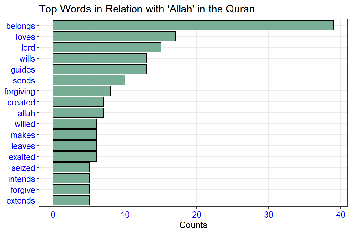
Figure 4.1: Top words with ‘Allah’ in the Quran
A bigram can also be treated as a term in a document in the same way that we treat individual words. For example, we can look at the tf-idf of bigrams across Surahs. These tf-idf values can be visualized within each long surah, just as we did for words in Chapter 2. This is shown in Figure 4.2.
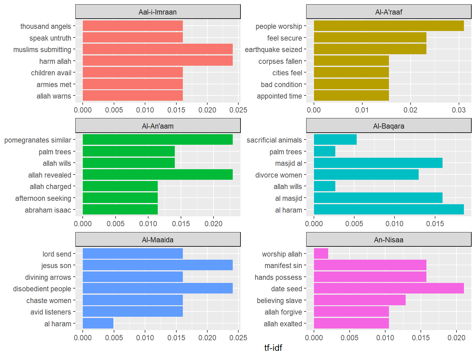
Figure 4.2: Top word pairs tf-idf in the long Surahs
There are advantages and disadvantages to examining the tf-idf of bigrams rather than individual words. Pairs of consecutive words might capture structure that isn’t present when we are just counting single words and may provide context that makes tokens more understandable (for example, “sacred house”, in Al-Maaida, is more informative than “house” or “sacred” separately). owever, the per-bigram counts are also sparser: a typical two-word pair is rarer than either of its component words. Thus, bigrams can be especially useful when you have a very large text dataset.
4.1.2 Visualizing a network of bigrams with ggraph
We may be interested in visualizing all of the relationships among words simultaneously, rather than just the top few at a time. One common visualization method is to arrange the words in a network graph. Here we will be referring to a “graph” as a combination of connected nodes. A graph can be constructed from a tidy object since it has three variables:
- from: the node an edge is coming from
- to: the node an edge is going towards
- weight: A numeric value associated with each edge
The igraph package has many powerful functions for manipulating and analyzing networks. One way to create an igraph object from tidy data is the graph_from_data_frame() function, which takes a data frame of edges with columns for “from” (word1), “to” (word2), and edge attributes (in this case n).
igraph has built-in plotting functions, but many other packages have developed better visualization methods for graph objects. The ggraph package (Pedersen 2017) implements these visualizations in terms of the grammar of graphics. We can convert an igraph object into a ggraph with the ggraph function, after which we add layers to it, much like adding layers in ggplot2. For example, for a basic graph, we need to add three layers: nodes, edges, and text.
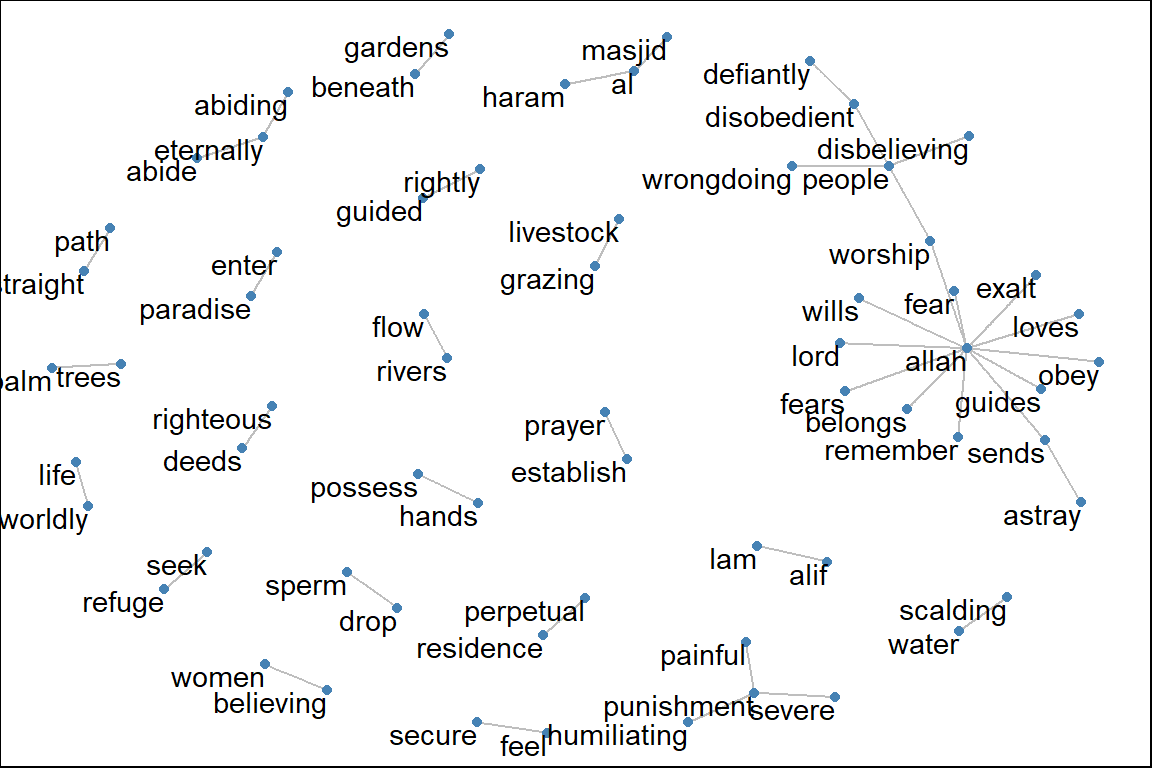
Figure 4.3: Common bi-grams in Saheeh
Figure 4.3 shows all the top bi-grams (count above 10) for Saheeh’s translation. From here we can make some observations, like the word “allah” having a dominant role, and some known concepts in Islam like “straight path” and “establish prayer”. “perpetual residence”, “rivers flow”, “gardens beneath” are known rewards for those who “enter paradise”.
We conclude with some polishing steps to make a nicer plot and at the same time reflect the attributes within the plot, such as re-sizing the edges to reflect the weights of the relations. The codes are presented below and the resulting plot is in Figure 4.4.
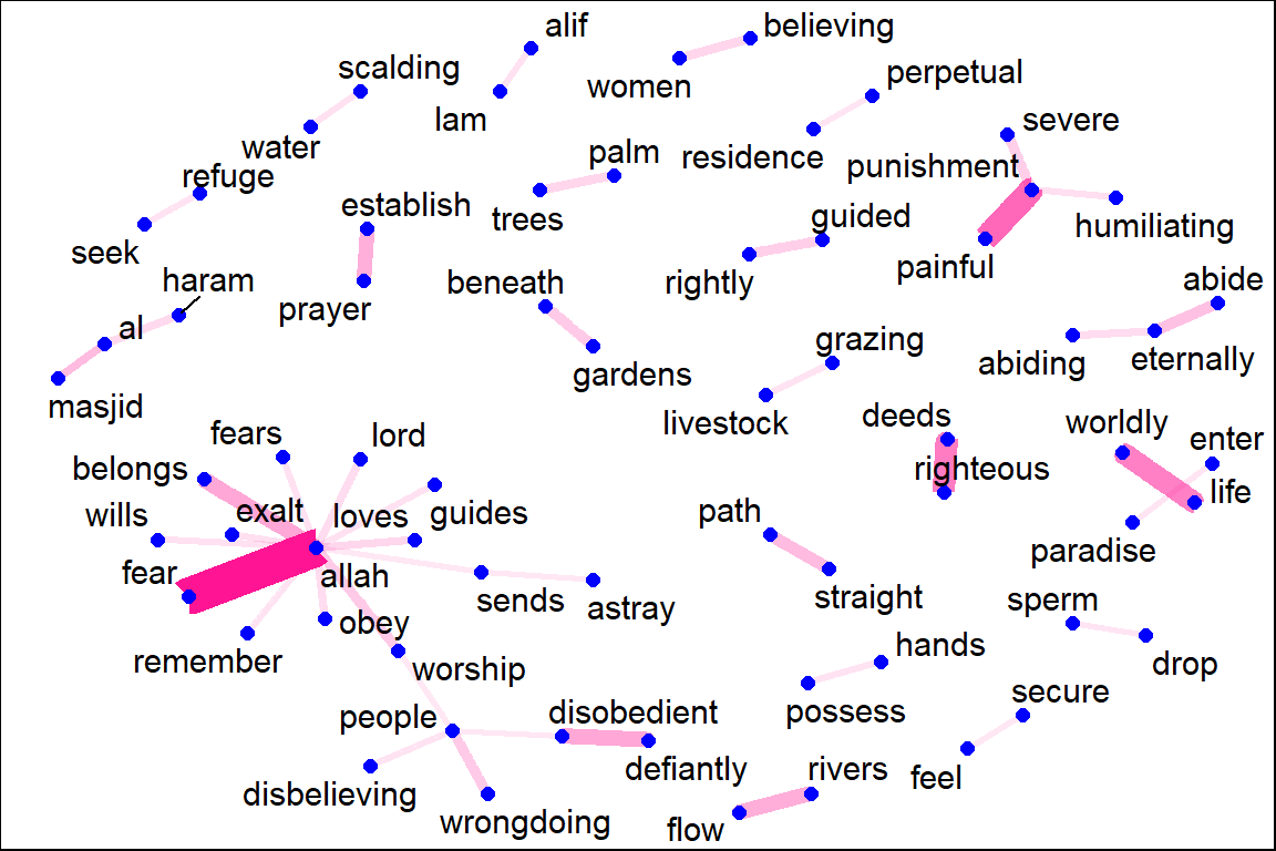
Figure 4.4: Common bi-grams in Saheeh with ggraph format
It may take some experimentation with ggraph to get your networks into a presentable format, but network visualization is a useful and flexible way to look at relational tidy data.
Note that this is a visualization of a Markov chain,49 a common model in text processing. In a Markov chain, each choice of a word depends only on the previous word. In this case, a random generator following this model might spit out “lord”, then “loves”, then “guides/obey”, by following each word with the most common words that follow it. To make the visualization interpretable, we chose to show only the most common word-to-word connections, but one can imagine an enormous graph representing all connections that occur in the Quran.
4.1.3 Tri-grams
We discuss next the most common trigrams, which are consecutive sequences of 3 words. We can find this by setting \(n = 3\) as shown in the code below:
ESI_trigram_counts <- quran_all %>%
  unnest_tokens(trigram, saheeh, token = "ngrams", n = 3) %>%
  separate(trigram, c("word1", "word2", "word3"), sep = " ") %>%
  filter(!word1 %in% stop_words$word,
         !word2 %in% stop_words$word,
         !word3 %in% stop_words$word) %>%
  count(word1, word2, word3, sort = TRUE)
ESI_trigram_counts <- ESI_trigram_counts %>%
                          filter(!is.na(word1) & !is.na(word2) & !is.na(word3))
ESI_trigrams_united <- ESI_trigram_counts %>%
                          unite(trigram, word1, word2, word3, sep = " ")
The result is viewed with:
## # A tibble: 6 × 2
##   trigram                          n
##   <chr>                        <int>
## 1 al masjid al                    16
## 2 masjid al haram                 15
## 3 defiantly disobedient people    10
## 4 people worship allah            10
## 5 firmly set mountains             9
## 6 alif lam meem                    8
Similar analyses performed for bigrams may be repeated for trigrams as well. We leave this subject for readers to try.
4.1.4 Bigrams co-ocurrences and correlations
As a next step, let us examine which words commonly occur together in the Surahs. We can then examine word networks for these fields; this may help us see, for example, which Surahs are related to each other.
We can use pairwise_count() from the widyr package to count how many times each pair of words occur together in a Surah.
word_pairs <- surah_wordsESI %>%
  pairwise_count(word, surah_title_en, sort = TRUE, upper = FALSE)
head(word_pairs)
Let us create a graph network of these co-occurring words so we can see the relationships better. The filter will determine the size of the graph.
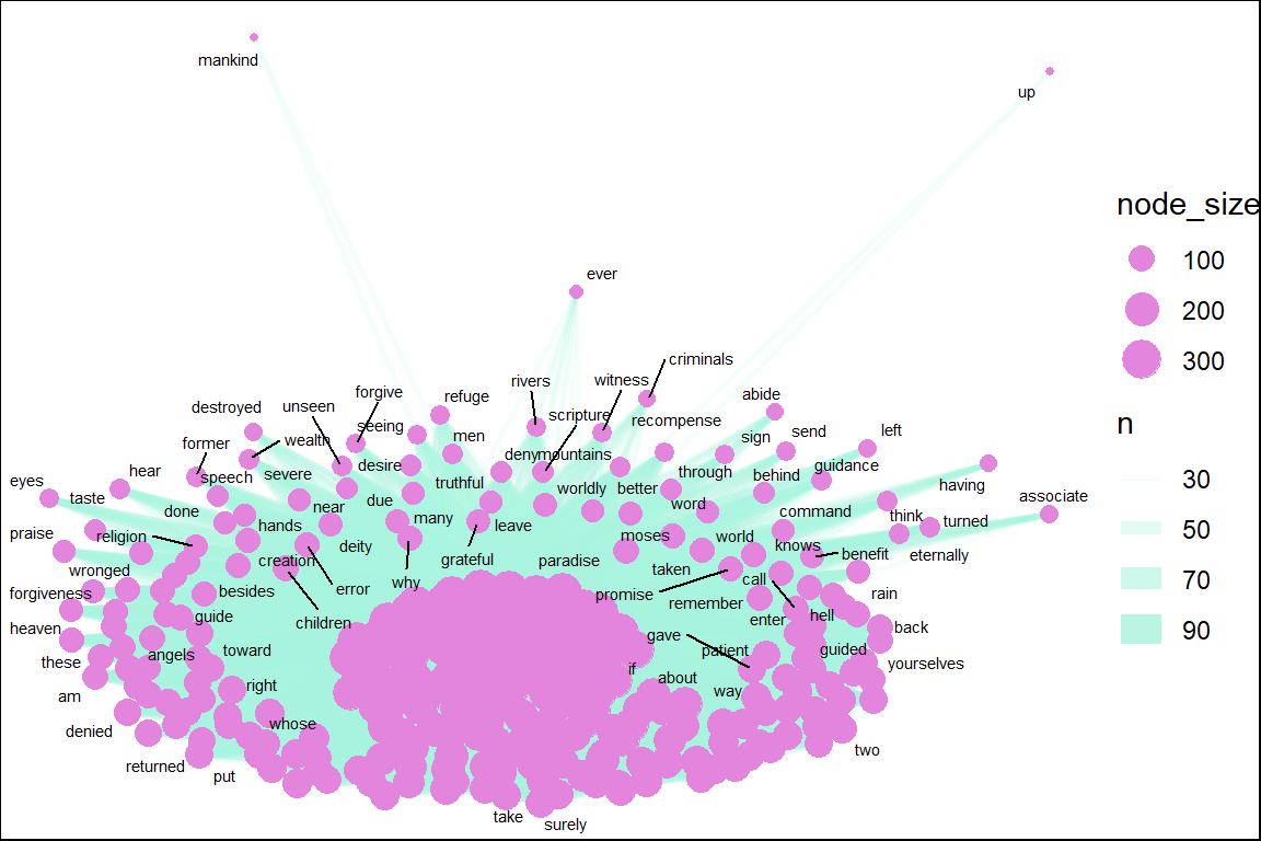
Figure 4.5: Common word pairs in Saheeh
Figure 4.5 exhibits the words (nodes) and their links (edges) to their pairs (other nodes) in the word pairs network for Saheeh. The size of the nodes indicates the degree of connections it has. The thickness of the links indicates the frequencies of links. At the center is the word “allah”, “lord” as expected. However, we can see many other words (nodes) such as “prayer”, which is highly linked to the center words (such as “allah”). Network visualization is a good starting point to make these types of observations.
4.1.5 Visualizing correlations of bigrams of keywords
Now we examine the relationships among keywords in a different way. We can find the correlation among the keywords by looking for those keywords that are more likely to occur together than with other keywords for a dataset.
keyword_cors <- surah_wordsESI %>%
  group_by(word) %>%
  filter(n() >= 50) %>%
  pairwise_cor(word, surah_title_en, sort = TRUE, upper = FALSE)
Let us visualize the network of keyword correlations.
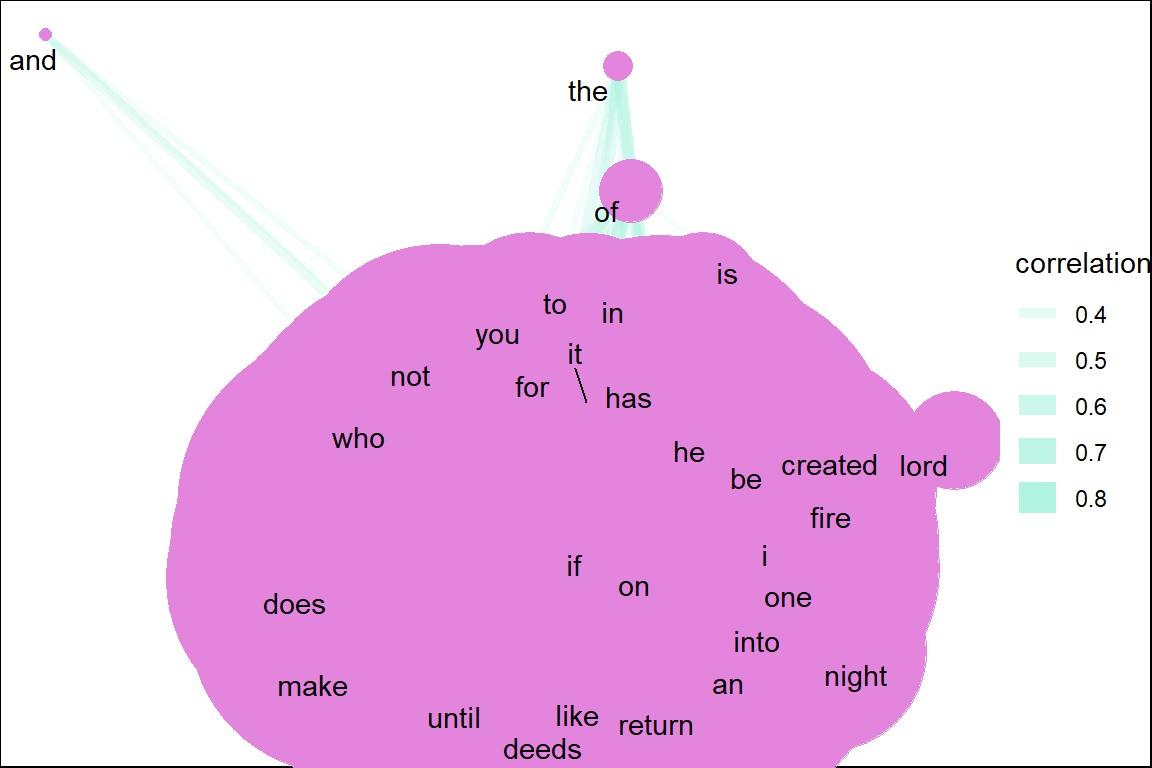
Figure 4.6: Common keyword correlations in Saheeh
From Figure 4.6, we can visualize all the keywords and their relations with other keywords. Note that the word “allah” and “lord” while being major keywords are less correlated to each other and other words. It shows that major keywords do not necessarily have high correlations with other keywords. This is the idea behind “keyword in context” (kwic) which we will cover in a later part of the book.
4.1.6 Summarizing ngrams
We have shown some methods of creating bigrams and analyzing them. Bigrams are the simplest relations between words, and the statistical properties of bigrams are rather straightforward. However, once we start to add more than two words, the complications grow exponentially. Let’s say that we have a window of five words (5-grams); what we have now is a space of four preceding words and four succeeding words, where the window is a moving window. Every time we move one word ahead, we move along the window and calculate the relations four steps backward and four steps forward. This is a very tedious and compute-heavy exercise. The same analyses done on bigrams explode into bigger scale computations when extended to a larger number of words and visual analyses are no longer possible.
Besides n-grams, we also have “skip-grams”. In skip-grams, instead of looking at words next to each other, we look at words within a distance to each other, such as three words away. Skip grams have their own purpose and use in analytics.
There are powerful algorithms used in NLP which utilize fast-speed mechanisms to convert words into compact vector representations. The development of these algorithms is to overcome computer memory problems, where when we have a large number of words in big corpora (such as the Internet), computing n-grams, skip-grams, will take too much memory space, and hence require compact space representations. This is especially when we want to apply learning models in Machine Learning algorithms such as Neural Network models.
4.2 Lexical analysis
An important NLP task in describing the relationships between words is lexical analysis. There are many good introductions to the subject, such as in Manning and Schutze (1999) and Manning, Raghavan, and Schutze (2009). The first step for lexical analysis involves Part-of-Speech (POS) tagging, stemming, and lemmatization.50 This is followed by syntactic parsing, which is the identification of words within grammatical rules (such as a verb, a noun, a phrase, etc.). Finally, the step involves dependency parsing, which is the process of analyzing the grammatical structure of sentences (i.e., the sequence of words in grammatical rules).
For lexical analysis processing, we deploy the udpipe package in R which was developed by Wijffels, Straka, and Straková (2020).51 For the purpose of demonstration, we select Surah Yusuf as our sample of analysis. The Surah is a fairly long chapter with 111 verses and mainly narrates the story of Prophet Yusuf (Joseph), which makes the analysis interesting.
We start with loading the udpipe language model for the English language, using the udpipe_download_model() function.
# During first time model download execute the below line too
# library(udpipe)
# udmodel <- udpipe_download_model(language = "english")
# Load the model
udmodel <- udpipe_load_model(file = 'data/english-ewt-ud-2.5-191206.udpipe')
We will start by annotating Surah Yusuf. The annotated data.frame is used for the analysis later.
Q01 <- quran_en_sahih %>% filter(surah == 12)
x <- udpipe_annotate(udmodel, x = Q01$text, doc_id = Q01$ayah_title)
x <- as.data.frame(x)
The resulting data.frame has a field called upos which is the Universal Parts of Speech tag and also a field called lemma which is the root form of each token in the text. These two fields give us a broad range of analytic possibilities.
4.2.1 Basic frequency statistics
In most languages, nouns (NOUN) are the most common types of words, next to verbs (VERB). These are the most relevant for analytic purposes, next to the adjectives (ADJ) and proper nouns (PROPN).52 The results of the frequencies are shown in Figure 4.7.
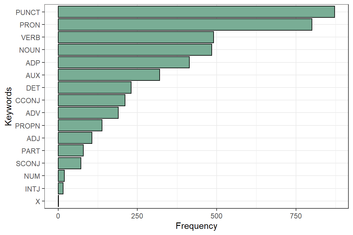
Figure 4.7: UPOS (Universal Parts of Speech) in Surah Yusuf
Parts of Speech (POS) tags allow us to extract easily the words we like to plot. We may not need stopwords for doing this, we just select nouns or verbs or adjectives and we have the most relevant parts for basic frequency analysis.
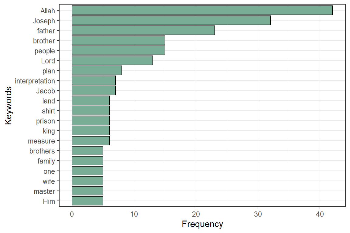
Figure 4.8: Most occurring nouns in Surah Yusuf
The NOUN and PROPN frequency plot in Figure 4.8 correctly reflect Allah (SWT) (also the words Lord, Him) as the central dominant subject matter of the Quran (Alsuwaidan and Hussin 2021). The noticeable noun missing in the plot is “prison”. The others are all recognizable to those familiar with Surah Yusuf. These are shown in Figure 4.9 and Figure 4.10.
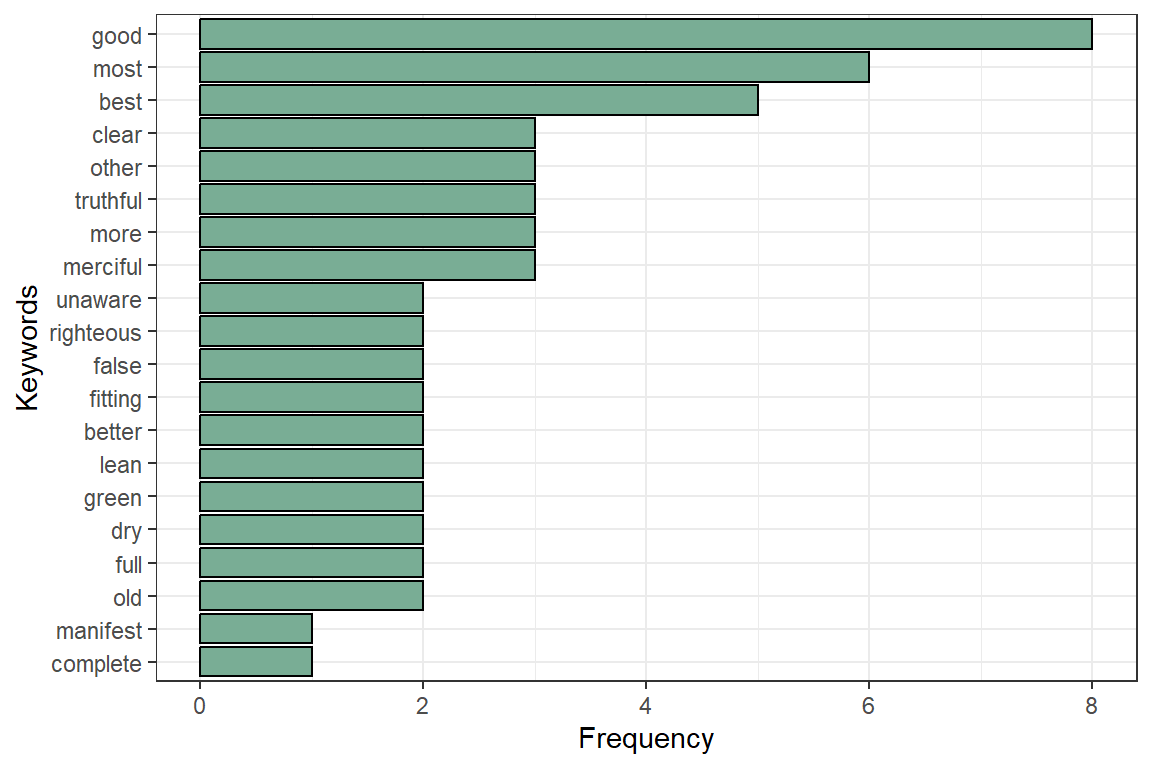
Figure 4.9: Most occuring adjectives in Surah Yusuf
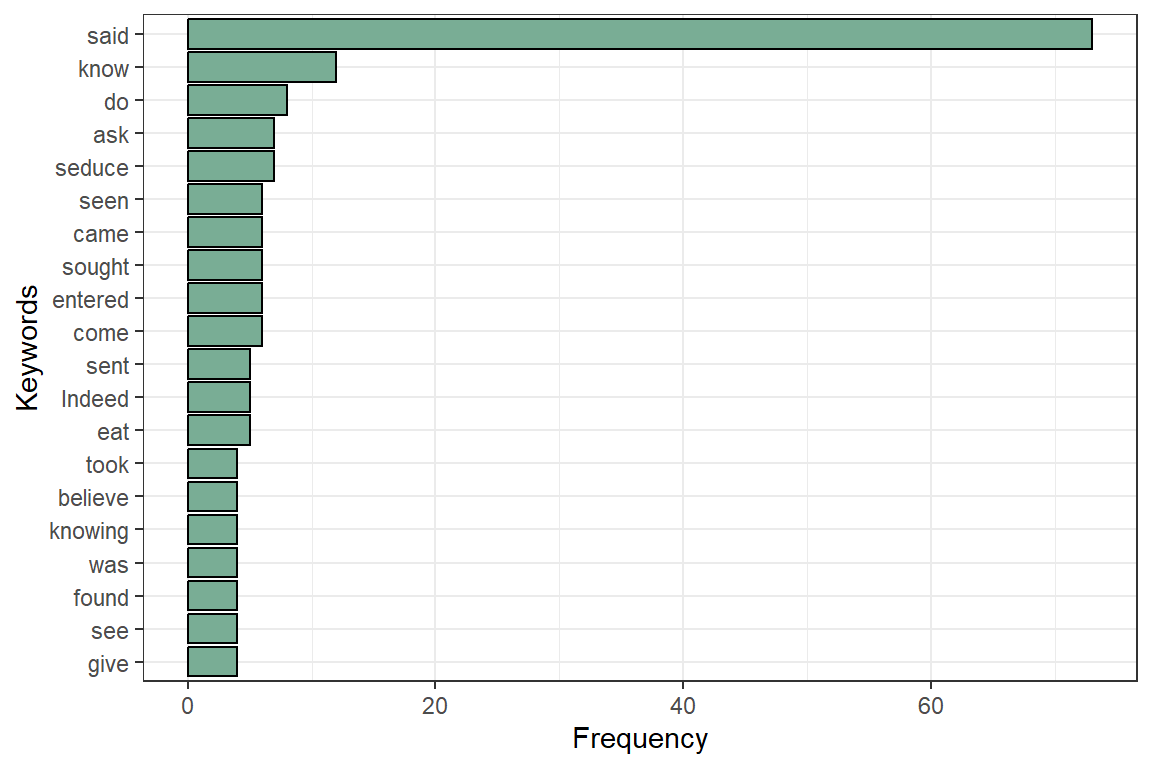
Figure 4.10: Most occuring verbs in Surah Yusuf
4.3 Word cooccurrences using POS
Analyzing single words is a good start. Multi-word expressions should be more interesting. We can get multi-word expressions by looking either at collocations (words following one another), at word co-occurrences within each sentence, or at word co-occurrences of words that are close in the neighborhood of one another.
Co-occurrences allow us to see how words are used either in the same sentence or next to each other. The udpipe package easily helps us create word co-occurrence graphs using the relevant POS tags.
4.3.1 Nouns, adjectives, and verbs used in same sentence
We look at how many times nouns, proper nouns, adjectives, verbs, and adverbs are used in the same sentence.
cooccur <- cooccurrence(x = subset(x, upos %in% c("NOUN", "PROPN", "VERB", "ADJ")),
                     term = "lemma",
                     group = c("doc_id", "paragraph_id", "sentence_id"))
The result can be easily visualized using the igraph and ggraph packages. This is shown in Figure 4.11.
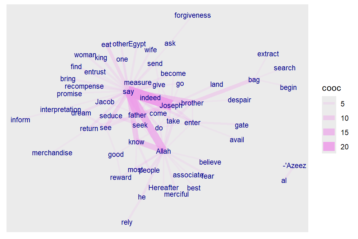
Figure 4.11: Co-occurence of Nouns, Names, Adjectives and Verbs
The story is revealed by Allah (SWT). The main characters are Joseph, his father, his brothers, the king, and the wife of the minister (al-’Azeez). So the verb “say” dominates since it is a narrated story. It is interesting to note the strong link and occurrence of “know” with “Allah”.
4.3.2 Words that follow one another using POS
Visualizing which words follow one another (bigram) can be done by calculating word co-occurrences of a specific POS type that follow one another and specify how far away we want to look regarding “following one another” (in the example below we indicate skipgram = 1 which means look to the next word and the word after that). Here we include the major POS.
cooccur <- cooccurrence(x$lemma,
              relevant = x$upos %in% c("NOUN", "PROPN", "VERB", "ADV", "ADJ"),
              skipgram = 1)
Once we have these co-occurrences, we can easily do the same plots as before. (See Figure 4.12).
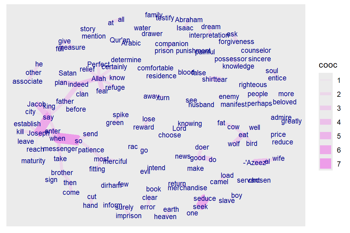
Figure 4.12: Words following one another in Surah Yusuf
4.3.3 Word correlations using POS
Keyword correlations indicate how terms are just together in the same document/sentence. While co-occurrences focus on frequency, correlation measures between 2 terms can also be high even if 2 terms occur only a small number of times but always appear together.
We show how nouns, proper nouns, verbs, adverbs, and adjectives are correlated within each verse of Surah Yusuf.
x$id <- unique_identifier(x, fields = c("sentence_id", "doc_id"))
dtm <- subset(x, upos %in% c("NOUN", "PROPN", "VERB", "ADV", "ADJ"))
dtm <- document_term_frequencies(dtm, document = "id", term = "lemma")
dtm <- document_term_matrix(dtm)
dtm <- dtm_remove_lowfreq(dtm, minfreq = 5)
termcorrelations <- dtm_cor(dtm)
y <- as_cooccurrence(termcorrelations)
y <- subset(y, term1 < term2 & abs(cooc) > 0.2)
y <- y[order(abs(y$cooc), decreasing = TRUE), ]
head(y)
## term1 term2 cooc
## 1126 seduce seek 0.7056591
## 681 eat other 0.6153136
## 1179 back shirt 0.5354312
## 1402 interpretation teach 0.4927311
## 49 bag brother 0.4850995
## 581 give measure 0.4298162The above pairings indeed reflect the story of Prophet Joseph.
4.4 Finding keyword combinations using POS
Frequency statistics of words are nice, but many words only make sense in combination with other words. Thus, we want to find keywords that are a combination of words. The steps here follow the example from An overview of keyword extraction techniques.53 The steps are as follows:
- by doing Parts of Speech tagging to identify nouns
- based on Collocations and Co-occurrences
- based on RAKE (Rapid Automatic Keyword Extraction)
- by looking for Phrases (noun phrases/verb phrases)
- based on the Textrank algorithm
- based on results of dependency parsing (getting the subject of the text)
Currently, the udpipe package provides three methods to identify keywords in text:
- RAKE (Rapid Automatic Keyword Extraction)
- Collocation ordering using Pointwise Mutual Information
- Parts of Speech phrase sequence detection
4.4.1 Using RAKE
RAKE is one of the most popular (unsupervised machine learning) algorithms for extracting keywords. It is a domain-independent keyword extraction algorithm that tries to determine key phrases in a body of text by analyzing the frequency of word appearance and its co-occurrence with other words in the text.
RAKE looks for keywords by looking to a contiguous sequence of words that do not contain irrelevant words by calculating a score for each word that is part of any candidate keyword. This is done by:
- among the words of the candidate keywords, the algorithm looks at how many times each word is occurring and how many times it co-occurs with other words.
- each word gets a score which is the ratio of the word degree (how many times it co-occurs with other words) to the word frequency.
A RAKE score for the full candidate keyword is calculated by summing up the scores of each of the words which define the candidate keyword. The result is in Figure 4.13.
stats <- keywords_rake(x = x,
            term = "lemma",
            group = "doc_id",
            relevant = x$upos %in% c("NOUN", "PROPN", "VERB", "ADV", "ADJ"))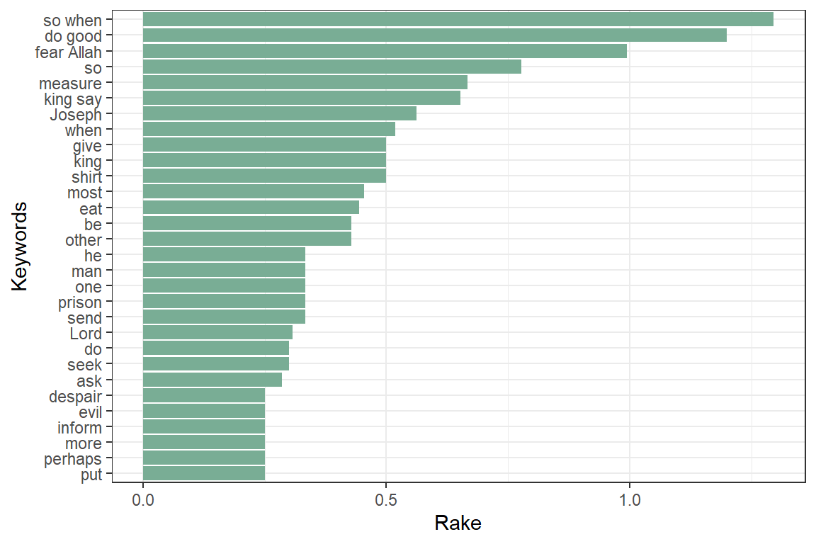
Figure 4.13: Keywords identified by RAKE in Surah Yusuf
4.4.2 Using Pointwise Mutual Information Collocations
The result is in Figure 4.14.
x$word <- tolower(x$token)
stats <- keywords_collocation(x = x, term = "word", group = "doc_id")
stats$key <- factor(stats$keyword, levels = rev(stats$keyword))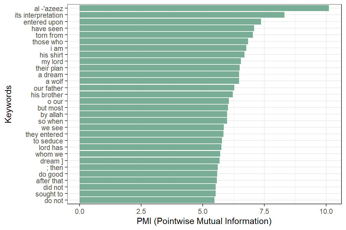
Figure 4.14: Keywords identified by PMI Collocation in Surah Yusuf
4.4.3 Using a sequence of POS tags (noun phrases)
Another option is to extract phrases. These are defined as a sequence of POS tags. Common types of phrases are noun phrases or verb phrases. In English, a noun and a verb can form a phrase like “Joseph said”. With the noun Joseph and verb said, we can understand the context of the sentence. We will show an example of how to extract noun phrases using the as_phrasemachine() function in udpipe.
POS tags are re-coded to one of the following one-letters:
- A: adjective
- C: coordinating conjunction
- D: determiner
- M: modifier of a verb
- N: noun or proper noun
- P: preposition
This simple example maps the various UPOS re-coded using letters.
y <- c("PROPN", "SCONJ", "ADJ", "NOUN", "VERB", "INTJ", "DET", "AUX", "NUM", "X", "PRON", "PUNCT", "ADP", "CCONJ")
as_phrasemachine(y)
We then define a regular expression to indicate a sequence of POS tags which we want to extract from the text. Extracting noun phrases from a text can be done easily by defining a sequence of UPOS tags. For example, this sequence of UPOS tags can be seen as a noun phrase: Adjective, Noun, Preposition, Noun. After which identifying a simple noun phrase can be just expressed by using the following regular expression (A|N)N(P+D(A|N)N) which says start with adjective or noun, another noun, a preposition, determiner adjective or noun and next to a noun again.54 The result is in Figure 4.15.
x$phrase_tag <- as_phrasemachine(x$upos, type = "upos")
stats <- keywords_phrases(x = x$phrase_tag, term = tolower(x$token),
                          pattern = "(A|N)*N(P+D*(A|N)*N)*",
                          is_regex = TRUE, detailed = FALSE)
stats <- subset(stats, ngram > 1 & freq > 3)
stats$key <- factor(stats$keyword, levels = rev(stats$keyword))
head(stats)
## keyword ngram freq key
## 28 those who 2 10 those who
## 29 his brother 2 9 his brother
## 31 my lord 2 9 my lord
## 33 our father 2 8 our father
## 39 which you 2 6 which you
## 46 his shirt 2 5 his shirt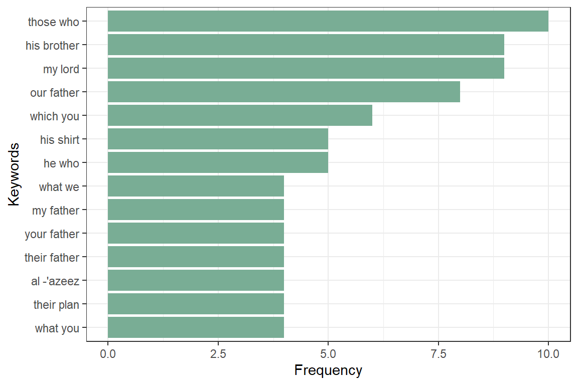
Figure 4.15: Keywords - simple noun phrases in Surah Yusuf
4.4.4 Textrank
Textrank is a word network ordered by Google Pagerank as implemented in the textrank (Wijffels and BNOSAC 2020) package.55 The algorithm allows to summarize text and extract keywords. This is done by constructing a word network by looking to see if words are following one another. On top of that network, the ‘Google Pagerank’ algorithm is applied to extract relevant words after which other relevant words which are following one another are combined to get keywords. In the example below, we are interested in finding keywords using that algorithm of either “NOUN”, “PROPN”, “VERB”, “ADJ” following one another.
stats <- textrank::textrank_keywords(x$lemma,
                  relevant = x$upos %in% c("NOUN", "PROPN", "VERB", "ADJ"),
                  ngram_max = 8, sep = " ")
stats <- subset(stats$keywords, ngram > 1 & freq >= 2)
head(stats)
## keyword ngram freq
## 7 he say 2 24
## 13 he brother 2 10
## 21 he have 2 6
## 22 have see 2 5
## 28 he shirt 2 4
## 32 eat he 2 3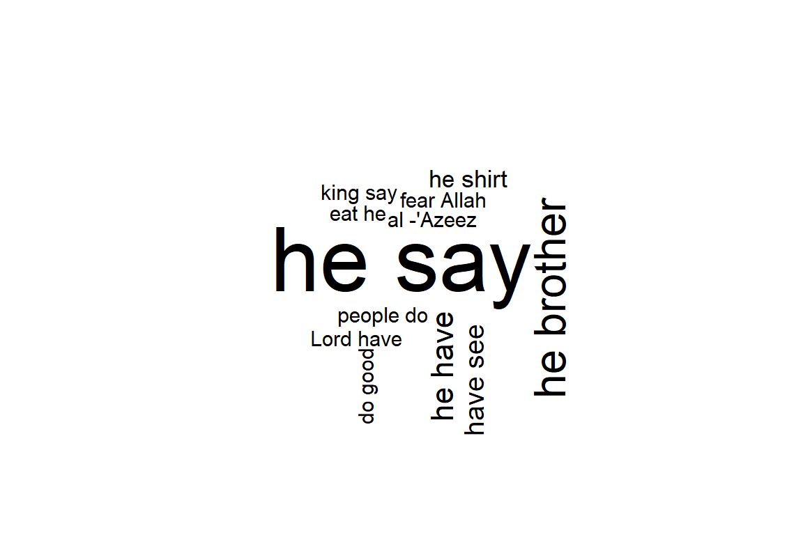
Figure 4.16: Textrank wordcloud for Surah Yusuf
Figure 4.16 shows that the keywords combine words into multi-word expressions. Again, we see the dominance of the verb “say” since Surah Yusuf is a narrated story. It is welcoming to note that “fear Allah” and “do good” are in fact the top moral lessons from this Surah.
“We relate to you the best of stories through Our revelation of this Quran, though before this you were totally unaware of them.” [12:3]
4.5 Dependency parsing
Finally, we address the subject of dependency parsing. Dependency parsing is an NLP technique that provides to each word in a sentence the link to another word in the same sentence, which is called the syntactical head. This link between every two words furthermore has a certain type of relationship giving us further details about it.
The udpipe package provides such a dependency parser. With the output of dependency parsing, we can answer questions like
- What is the nominal subject of a text
- What is the object of a verb
- Which word modifies a noun
- What is the link to negative words
- Which words are compound statements
- What are noun phrases, verb phrases in the text
Here we use the dependency parsing output to get the nominal subject and the adjective. When we executed the annotation using udpipe, the dep_rel field indicates how words are related to one another. A token is related to the parent using token_id and head_token_id. The dep_rel field indicates how words are linked to one another. The type of relations is defined on the Universal Dependencies website.56 Here we are going to take the words which have a dependency relation nsubj indicating the nominal subject and we are adding to that the adjective which is changing the nominal subject.
In this way, we can combine what the Surah is talking about with the adjective or verb it uses when it describes a subject.
stats <- merge(x, x,
           by.x = c("doc_id", "paragraph_id", "sentence_id", "head_token_id"),
           by.y = c("doc_id", "paragraph_id", "sentence_id", "token_id"),
           all.x = TRUE, all.y = FALSE,
           suffixes = c("", "_parent"), sort = FALSE)
stats <- subset(stats, dep_rel %in% "nsubj" &
                  upos %in% c("NOUN", "PROPN") &
                  upos_parent %in% c("VERB", "ADJ"))
stats$term <- paste(stats$lemma, stats$lemma_parent, sep = " ")
stats <- udpipe::txt_freq(stats$term)
data.frame("keyword"= stats$keyword,"left" = stats$left,
           "right"= stats$right, "pmi" = stats$pmi )
## data frame with 0 columns and 0 rowsWe can visualize the dependency in a wordcloud plot.
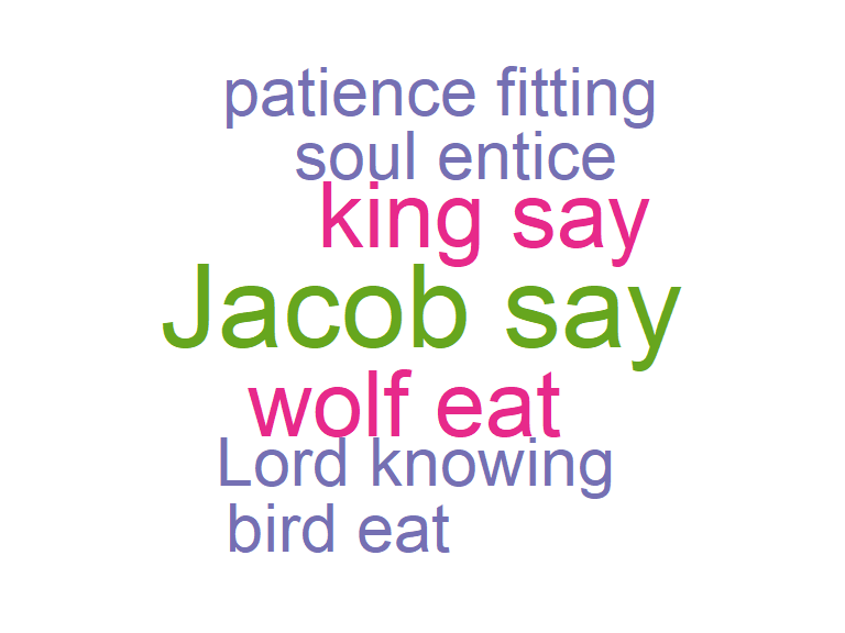
Figure 4.17: Dependency parsing wordcloud for Surah Yusuf
The plot in Figure 4.17 confirms the comment we made earlier about “say”. Another known moral lesson from Surah Yusuf, “patience fitting”, now appears. We have shown how to use the dep_rel parameter that is part of the annotation output from the udpipe package. For visualizing the relationships between the words which were found, we can just use the ggraph package. Now we introduce a basic function that selects the relevant columns from the annotation and puts it into a graph as guided by Wijffels, Straka, and Straková (2020) 57. The code for the function is reproduced as a reference in the Appendix at the end of the chapter.
We can now call the function as follows to plot verse 12:16 in Surah Yusuf. See Figure 4.18. And a longer verse, verse 12:31. (See Figure 4.19).
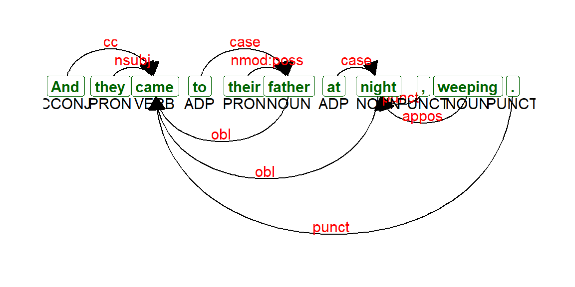
Figure 4.18: Dependency parsing udpipe output Verse 12:16

Figure 4.19: Dependency parsing udpipe output Verse 12:31
With dependency parsing, we can now see, for example, how nouns relate to the adjectives with nominal subject as the type of relationship.
4.5.1 Collocations and co-occurences
Once we have performed the dependency parsing (i.e., all the taggings) for the corpus (or selected subset within the corpus), we can redo all the exercises done in the earlier part of the chapter; namely the collocation measures of “n-grams”, “skip-grams”, and the co-occurrence measures such as words correlations, and fitting them into a network.
Now that we have classified each word as “NOUN”, “PRONOUN”, “VERB”, etc., we can perform the exercises such as collocations among nouns and pronouns, between verbs, or combing noun and verbs. The permutations are almost limitless. Since our intent is only to introduce the subject and the tools available, we will leave it for researchers with a background in linguistics.
4.6 Summary
This initial exploration of the udpipe package with just one of the 114 Surahs in Saheeh translation of Al-Quran has indeed shown some interesting and unique analysis. The results confirm many familiar lessons for those acquainted with the Quran and Surah Yusuf, in particular.
The study also opens other investigation avenues like
- Looking into other Surahs of the Quran,
- Other translations,
- Other use cases of udpipe,
- Most importantly, analyzing the original Arabic Quran.
The first in the “to-do” list should be easy since the codes can be repeated by just changing the selected Surah to analyze. We encourage our readers to pursue this.
The second can also be easily tested with other English translations of the Quran like what we have shown in Chapter 2 and Chapter 3. Again, we leave this to our readers. It can also be repeated with translations of the Quran in other languages that are supported by udpipe.58
We will explore the third item in the coming chapters. The final “to-do” item is massive and extremely valuable. We must define a full project scope for it. Applying the NLP tools that we have covered so far is the easier part, but interpreting the results will be the real challenge. Much of this work has been done by Corpus Quran project59; the work of which still requires intensive development and verification of its accuracies and appropriateness.60
In the next chapter, we will go deeper into the tools of network graphs in R. We have used it quite heavily in this chapter and in some of the earlier chapters. Our work on Quran Analytics will use these tools frequently. As such, a simple tutorial on these tools using examples from the Quran should be useful.
4.7 Further readings
widyr package in R. (Robinson, Misra, and Silge 2020)
udpipe package in R. (Wijffels, Straka, and Straková 2020)
tm package in R. (Feinerer, Hornik, and Software 2020)
textrank package in R. (Wijffels and BNOSAC 2020)
Appendix
Function for Udpipe Dependency Parser output
The codes for this function was produced by bnosac (https://www.bnosac.be).
plot_annotation <- function(x, size = 3){
  stopifnot(is.data.frame(x) &
            all(c("sentence_id", "token_id", "head_token_id",
                  "dep_rel", "token", "lemma", "upos",
                  "xpos", "feats") %in% colnames(x)))
  x <- x[!is.na(x$head_token_id), ]
  x <- x[x$sentence_id %in% min(x$sentence_id), ]
  edges <- x[x$head_token_id != 0,
             c("token_id", "head_token_id", "dep_rel")]
  edges$label <- edges$dep_rel
  g <- graph_from_data_frame(
              edges,
              vertices = x[, c("token_id", "token",
                               "lemma", "upos", "xpos", "feats")],
              directed = TRUE)
  ggraph(g, layout = "linear") +
      geom_edge_arc(
        ggplot2::aes(label = dep_rel, vjust = -0.20),
        arrow = grid::arrow(length = unit(4, 'mm'),
                            ends = "last",
                            type = "closed"),
        end_cap = ggraph::label_rect("wordswordswords"),
        label_colour = "red", check_overlap = TRUE, label_size = size) +
      geom_node_label(ggplot2::aes(label = token),
                      col = "darkgreen",
                      size = size, fontface = "bold") +
      geom_node_text(ggplot2::aes(label = upos), nudge_y = -0.35, size = size) +
      theme_graph(base_family = "Arial Narrow") +
      labs(title = "udpipe output",
         subtitle = "tokenisation, parts of speech tagging & dependency relations")
}
References
Language model developed by the Institute of Formal and Applied Linguistics, Charles University, Czech republic.↩︎
A comprehensive textbook on n-gram models is (Manning and Schutze 1999).↩︎
A Markov chain is a mathematical system that experiences transitions from one state to another according to certain probabilistic rules. The defining characteristic of a Markov chain is that no matter how the process arrived at its present state, the possible future states are fixed. https://brilliant.org/wiki/markov-chains/↩︎
The goal of both stemming and lemmatization is to reduce inflectional forms and sometimes derivationally related forms of a word to a common base form.↩︎
The udpipe model is developed by the Institute of Formal Applied Linguistics, Charles University, Czech republic. Guides for using the package are available at (https://bnosac.github.io/udpipe/docs/doc5.html)↩︎
For a detailed list of all POS tags, please visit https://universaldependencies.org/u/pos/index.html↩︎
https://www.r-bloggers.com/2018/04/an-overview-of-keyword-extraction-techniques/↩︎
https://www.rdocumentation.org/packages/udpipe/versions/0.8.5/topics/keywords_phrases↩︎
https://cran.r-project.org/web/packages/textrank/index.html↩︎
http://www.bnosac.be/index.php/blog/93-dependency-parsing-with-udpipe↩︎
https://cran.r-project.org/web/packages/udpipe/vignettes/udpipe-annotation.html↩︎
Accuracies of the work is still a work in progress, as claimed by the developers, posted on its message board (https://corpus.quran.com/messageboard.jsp)↩︎