7 Texts Network Analysis
Natural Language Processing (NLP) is a combination of linguistics and data science analyzing large amounts of natural language data which includes a collection of speeches, text corpora, and other forms of data generated from the usage of languages. The tasks of NLP vary from text mining and speech recognition (data-driven) to more complex tasks such as automatic text generation or speech production (AI-driven).
In this chapter we will focus on one particular aspect of NLP applied to a chosen text of the English translation of the Quran, namely lexical semantic analysis. This analysis focuses on what is termed as individual words in context analysis. Lexical semantics is the study of word meanings within its internal semantic structure or the semantic relations that occur within the corpus.78 We will focus on the second approach, namely to study words in relation to the rest of the words in the complete text, in this case, the Saheeh English translation of Al-Quran.
We will also take a very specific approach by deploying network graphs (or properly known as graph theory). We start with visualization of words within the text as a network of relations (words in the text as nodes and their presence in a sentence as directed edges). Relationships can take several forms to suit a particular interest. It may be to discover main messages in the text or analytical reasoning such as to uncover the major topics within those messages. It can be explorative analysis, such as how these messages and topics relate to each other within the main message (or text).
Another important point to mention is the difference between the parametrical and non-parametrical approach to the task at hand. The parametrical approach relies on some pre-built models, such as sentiment scoring, semantic ontologies, etc. The non-parametric approach does not rely on any models and instead will be driven by the empirical nature of the words and the text itself (i.e. do not rely on other samples from outside of the sample at hand). We will use the second approach by using network analysis and graph theory.
In network analysis, identifying a few methods will help greatly. An example is the formation of the network whether it follows a random graph or any particular graph structure. Another important issue is on the emergent structures, whether any emergent structure can be observed, and if it exists, we can uncover the factors of the emergent structures and sub-structures. This will bring us into the subject of complicatedness and complexity of systems analysis. Given the enormous possibilities and size of the task, this chapter will focus on providing preliminary findings using basic network analysis. We will identify some open issues for future work. To perform the various analysis, we will use two main packages in R, namely quanteda (Benoit et al. 2018) and igraph (Csárdi 2020). Quanteda is a complete suite of R packages for text analytics with many ready-made built-in functions that are easy to use. iGraph is a network (or graph network) package in R. Both packages are well developed and supported within the R programming community. For the data, we will use the prebuilt text in tidydata format from quRan package, and for some of the utilities required, we will use the quanteda package. For purposes of fast computation and visualization of a large network, we will use open-source software, Gephi . Similar software are Pajek , Cytoscape , and NodeXL . As far as computation is concerned there are no additional advantages offered by these software applications, except for easier visual manipulation and production of images. We will rely on Gephi for this purpose while using R as our main engine for computations.
7.1 A brief on quanteda
The work for this chapter and the next relies on the quanteda package; hence we feel it is appropriate to present a short and brief tutorial on the package (as we have done for tidytext, igraph, and ggraph in earlier chapters).
The quanteda package is among the recent introductions into the family of NLP tools in R. It was developed by Kenneth Benoit and many developers, supported by the European Research Council(Benoit et al. 2018). The package contains comprehensive text modeling functions from start to end - which includes basic features from tokenization to unsupervised learning models of text analysis.79
quanteda has four basic types of objects:
- corpus() which is corpus, the collection of texts in textual format.
- tokens() which is a tokenizing function, the tokens for the texts with all the metadata and tagging
- dfm() a Document-feature matrix (DFM), a document-term-matrix, which is a sparse matrix of 0 and 1, indicating the occurrence of a term in a document (which is a sentence or set of texts)
- fcm() a Feature Co-occurrence Matrix (FCM), a term-to-term-matrix, which is a sparse matrix of 0 and 1, indicating co-occurrence of a term with another term, within the entire document or corpus.
In most text analytics packages, the first three objects are available directly from the package, while the feature’s matrix is generated from pre-processing exercises before being fed onto a learning model. The advantage of quanteda is fast and seamless processing or creation of the FCM.
Text analysis with quanteda goes through all these four types of objects either explicitly or implicitly.
corpus()
Once a corpus is created, we can manipulate the corpus with many functions. corpus_reshape() is an important tool for converting data from long to wide format. Subsetting of a corpus is done via corpus_subset(). corpus_segment() allows us to select documents in a corpus based on document-level variables. Trimming the corpus is through corpus_trim().
tokens()
To create tokens from a corpus or text data, we use the tokens() function, which will create a tokenized dataset, consisting of tokens object. Once we have the tokens object, we can manipulate it with many ready-made functions, such as tokens_lookup() for quick search of tokens, tokens_subset(), tokens_sample(), tokens_split() for creating subsets the tokens; _tokens_select(), tokens_replace(), which are an important tool for replacing or changing items inside the tokens object; and finally, tokens_remove(), tokens_tolower(), tokens_wordstem() for manipulating the tokens object.
char()
There are also character-level manipulation functions that serve general utility purposes. These are: char_tolower(), char_toupper(), char_ngrams(), char_select(), char_remove(), char_keep(), char_trim(), etc. They are all are similar to the methods used in tidytext character manipulations functions.
dfm()
Document Feature Matrix object is created by dfm() function. This is among the major objects in quanteda. It is a sparse matrix with named rows and columns. The names for the rows are the document labels, and the names for the columns are the features (or tokens). Once created, we can use dplyr like functions such as dfm_group() for group-by, dfm_select() for selecting tokens, dfm_remove() for removing tokens, dfm_sort() for sorting, and so on.
fcm()
Feature Co-occurrence Matrix object is created by fcm() function. It is a square sparse matrix with named rows and columns. The names for the rows and the columns are the features (or tokens). Once created, the manipulations are similar to the dfm object, where we can use functions such as fcm_select() for selecting tokens, fcm_remove() for removing tokens, fcmm_sort() for sorting, and so on.
Utility functions
There are a few useful functions to apply on dfm or fcm objects, which are handy, such as docfreq() for calculating frequencies of the tokens, and topfeatures() for getting the top features. General ones include: ndoc(), nfeat(), nsentence(), ntoken(), ntype() for counting purposes. One of the less well-known, but powerful functions is dictionary(), which creates a dictionary type data, which is handy for dealing with large amounts of text data, when generating vocabulary is required. The dictionary object can be manipulated easily with dictionary_edit(), char_edit(), and coercion between objects is by using the as.dictionary() function.
Network and plotting functions
Creating and converting objects into networks, and plotting is a cumbersome process. quanteda makes this easy by a seamless process of converting dfm or fcm object into an igraph object, which then can be used for graph manipulations and calculations. It also creates few wrappers around the ggplot2 functions for easy plotting of network objects. An example of such functions is textplot_network().
statistical functions
The statistical functions are named as textstat_xxx(). They are textstat_simil() for texts similarity calculations, textstat_dist() for texts distance measures, textstat_frequency(), textstat_keyness(), textstat_collocation(), textstat_entropy(), and numerous others. All of these functions are extremely useful for quick calculations of the statistical measures which are available for usage in analysis.
quanteda textmodels
As an extension to the brief on quanteda, we introduce the quanteda.textmodel package. It is a dedicated suite for text modeling work, which has many applications for running statistical learning models - taking advantage of the data structure of quanteda objects. There are many models developed include textmodel_wordscores(), text_model_affinity(), textmodel_svm() (Support Vector Machines), textmodel_nb() (Naive Bayes), textmode_lsa(), and others. We will describe the models in the next chapter (Chapter 8).
R code examples of using quanteda are given below:
library(quanteda)

# create a corpus
corp_kahf <- corpus(quran_en_sahih)
corp_kahf_sub <- corpus_subset(corp_kahf,ayah >= 100)

# tokenize and process
toks_kahf <- quanteda::tokens(corp_kahf,remove_punct = TRUE) %>%
              tokens_tolower() %>% tokens_remove(pattern = stop_words$word,
                                                padding = FALSE)

# create dfm and fcm using tokens or corpus
dfm_kahf <- dfm(toks_kahf); dfm_kahf <- dfm(corp_kahf)
fcm_kahf <- fcm(toks_kahf); fcm_kahf <- fcm(corp_kahf)

# dfm and fcm manipulations
dfm_kahf_sub <- dfm_subset(dfm_kahf, surah_title_en == "Al-Baqara")
fcm_kahf_sub <- fcm_select(fcm_kahf, pattern = c("allah","lord"))

# using dictionary
dict <- dictionary(list(god = c("allah","lord"),
                prophet = c("prophet","muhammad","moses")))
dfm(corp_kahf, dictionary = dict)
For the rest of this chapter, we will utilize the quanteda package and work through our analysis utilizing the various functions for the dual purpose of providing a tutorial and applying them to specific examples.
7.2 Analyzing word cooccurrence as a network
7.2.1 Network dynamics: growth of word co-occurrence network
In network analysis, an important aspect is the dynamics of the network growth, from a few nodes and edges until it becomes a full-blown network. This phenomenon is important in network analysis, whereby a network may start as a small set, and over time it grows into its full size. In the words network, it may start with a few central words (or vocabulary) and as more words are added to the network, it will grow into a full network of words.
For the Saheeh English Quran, how does this growth behavior look like? This is the question we want to investigate. From the start, we know that the most frequent (and hence central word) is “Allah”. How do other words start to attach to this central “node”, as we increase the words by the order of frequencies?
quran_all = read_csv("data/quran_trans.csv")
tokensQ = quran_all$saheeh %>%
      tokens(remove_punct = TRUE) %>%
      tokens_tolower() %>%
      tokens_remove(pattern = stop_words$word, padding = FALSE)
dfmQ = dfm(tokensQ)
fcmQ <- fcm(tokensQ, context = "window", tri = FALSE)
fcm_tpnplot = function(fcmQf,n,vls){
  feat <- names(topfeatures(fcmQf, n))
  fcmQ_feat <- fcm_select(fcmQf, pattern = feat)
  v_size = rowSums(fcmQ_feat)/min(rowSums(fcmQ_feat))
  fcmQ_feat <- fcm_select(fcmQ, pattern = feat)
  fcmQ_feat %>%
    textplot_network(min_freq = 0.5,
                edge_color = "gold",
                edge_alpha = 0.5,
                edge_size = 2,
                vertex_size = 1,
                vertex_labelsize = vls*log(v_size))
}
p1 = fcm_tpnplot(fcmQ, n = 10,vls = 2)
p2 = fcm_tpnplot(fcmQ, n = 20,vls = 1)
p3 = fcm_tpnplot(fcmQ, n = 50,vls = 0)
p4 = fcm_tpnplot(fcmQ, n = 200,vls = 0)
cowplot::plot_grid(p1,p2)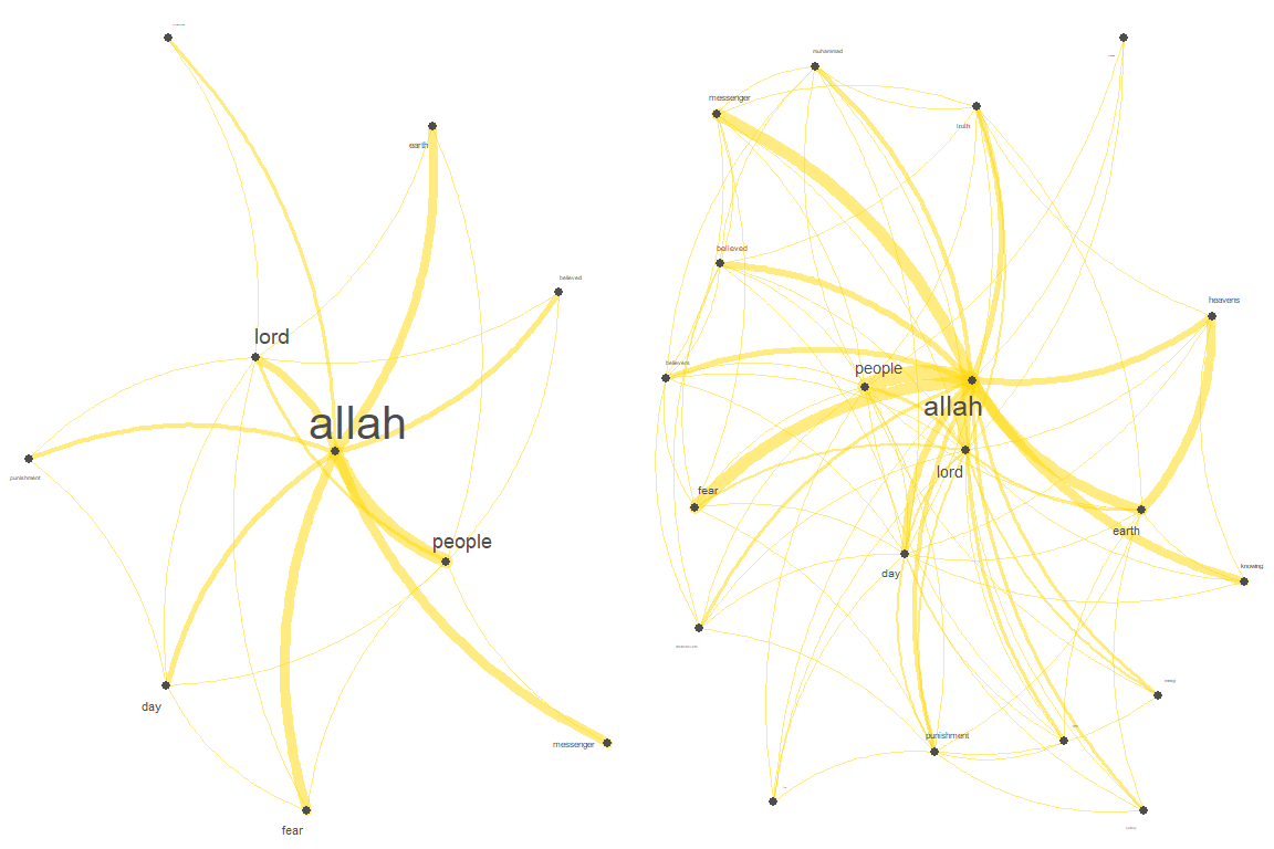
Figure 7.1: Growth of words co-occurrences network in Saheeh
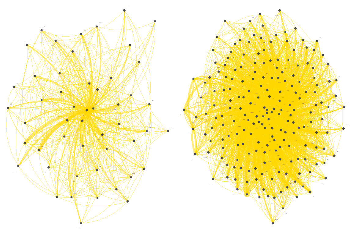
Figure 7.2: Growth of words co-occurrences network in Saheeh
Figure 7.1 shows the network growing from 10 to 20 words; and Figure 7.2 is from 50 to 200 words.
We can observe that the word network grows centrally from the single word “Allah”, and it grows in a particular way as more words are added until the network is dense. More importantly, the whole word network (for co-occurrence network) is “one” single large network, densely organized. This is an important observation. The question is what does it mean?
Here we enclose a sample of a full-blown word co-occurrence network from the novel Moby Dick (Chapter 1) as a comparison (in Figure 7.3). It is a fully connected network, forming a single large network, but the network is not as dense as the network shown for Saheeh. In fact, if we do a similar step of checking the growth of the network, it is not the same as what we see in Saheeh.80
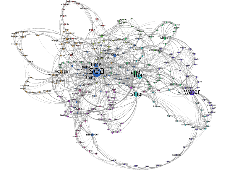
Figure 7.3: Example of co-occurrence network in Chapter 1 of Moby Dick novel
Furthermore, a detailed look at the plot (which is not shown here) reveals that the early keywords seem to have some “themes” to it; namely about “allah”, “lord”, “believe”, “day”, “people”, “muhammad”, “messenger”, and the themes grow out of these main themes. While these themes grow, the centrality of “allah” remains and grows stronger as the network size expand. This is termed the “emergent structure” of the network. Why this is true, is a subject that requires further research and analysis, which we encourage readers to pursue.
And if we expand to all co-occurrences on the entire Saheeh corpus, we will get the picture in Figure 7.481, which is amazingly interesting.
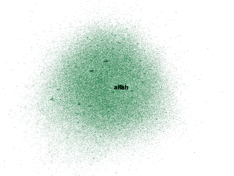
Figure 7.4: Saheeh entire corpus word co-occurence network
The center of the network remains singly to “allah”, and a zoomed view to the center is shown in Figure 7.5, which shows the central node, and all other major nodes (i.e., themes) - which are ordered as “allah”, “lord”, “people”, “day”, and so on. These “themes” interestingly coincide with the major “subject matters” as discussed by one of us through a qualitative analysis of the Quran.
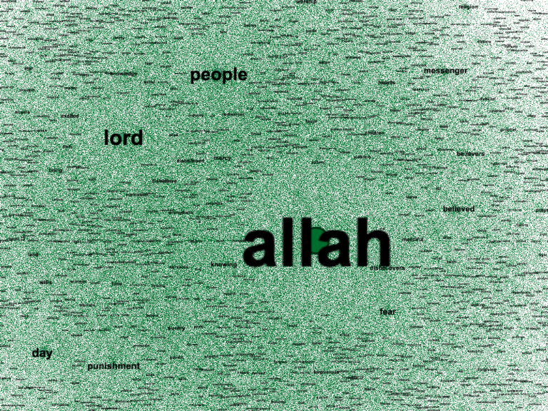
Figure 7.5: Close up view of the center of the network
7.2.2 Word co-occurrence network statistics
The word co-occurrence network is about understanding how each word that appears in the text relates to all other words which appear in the whole text. The connections or links between the words explain the structure of the messages or topics of the texts. The example in Figure 7.3 is a word co-occurrence network for Chapter 1 of Moby Dick’s novel. It shows the whole text is centered around “sea” and “man”, and sub-grouped by “water”, “ship”, and “voyage”. The colors of the nodes represent sub-groupings (or cliques) whereby such sub-groupings may represent another message or sub-topic by themselves. The same process happens in growing the network shown in Figure 7.3 for Saheeh’s entire corpus.
Now let us work using the igraph package and explore various statistical analyses using graph theory in understanding the network.
First let us get the number of words (nodes) and co-occurrences (edges) in the whole word co-occurrence network (graph).
## [1] "nodes = 4801 and edges = 267668"There are 4,801 words (nodes) and 267,668 edges in the network. Note that we have removed all the stop-words, which otherwise will confound the network with all the stopwords in between. Recall that from Chapter 5, we have recorded that the total unique tokens (words) for Saheeh is 5,739 (including stopwords). Almost one thousand tokens are not present, due to either being removed as stopwords or the tokens have zero co-occurrence, and hence not included.
There are a few general statistics that we are interested in, namely: diameter, paths and distance, connectedness, clustering, and modularity measures of the network. The previous chapter introduced a basic tutorial on these measures using a smaller word co-occurrences network graph from just one Surah. We now extend applying the same concepts for the entire Saheeh Quran corpus.
7.2.3 Diameter and average distance
In a network, the diameter is the measure of the “longest span”, which implies the maximum “hops” or “steps” it takes from one node to reach the furthest node from it. This is also called the measure of “small-world properties” of Watts-Strogatz.82 In a word network, it means how many words in between that it will take for a word to be connected to another word.
So how many words in between, for it to be connected to the furthest word in Saheeh? The answer is 6 words. How do we make sense out of this number? As a comparison, the network diameter for the internet is 6.98 and the E.coli metabolism network has a diameter of 8. Comparing with English texts (such as novels or textbooks) the “normal diameter” is between 10 to 14, and the measure is about the same for a few other Latin-based languages.83 What we are observing here is a phenomenal structure, a corpus of English text having a measure of diameter much smaller than any normal texts, and extremely close to the measures of the network in nature (e.g., E.Coli protein network).
Average distance is a measure of “halfway” steps needed to reach the “center” of the network. The measure for Saheeh is 2.55. The comparable number for English books is between 3.33 to 3.60. Again, in our case here we can say that any word is not more than 2.55 steps away on average from the center word, which is “Allah”, the central theme.
What all of these measures mean is that the word network for Saheeh exhibits similarities to the Small World network! In fact, for an Erdos-Renyi (random graph) network, the comparable numbers are between 14 to 20 for the diameter and between 4.60 to 6 for the average distance.(Ban, Meštrović, and Martincic-Ipsic 2014) This means that the words co-occurrences in Saheeh are not random in nature, and in fact well structured as a dense network.
These properties very strongly indicate how closely related are all the words in Saheeh and the conciseness of the sentences in the text. Lower diameters and average distances are good measures of “efficiencies” in a large network. In the case of Saheeh, the measures clearly imply that the words in the texts are used with extreme efficiency.
7.2.4 Connectedness
Measures of connectedness reflect the components of the network, whether the network consists of a single large component or separated into few components. The codes below compute these measures:
## [1] 9## [1] 4783 2 2 2 3 2 3 2 2The result shows that there are 9 components, and in fact the single largest component (giant component) consists of 4,783 nodes, which is 99.63% of the total nodes. This shows that the network is actually a single giant component, and it is also a fully connected network, which means that there is no single word that is not related to at least another word. It also implies that the whole network (i.e. every word) has a relation (directly or indirectly) with every other word in the network.84
7.2.5 Degree distributions
A degree is a link between two words, and the total number of links attached to a word is called the degree of the node (word). We are interested how does the degree for the entire nodes in the network loos like, from a statistical distributions perspective.
The codes below compute the degree for the Saheeh network and plot them.
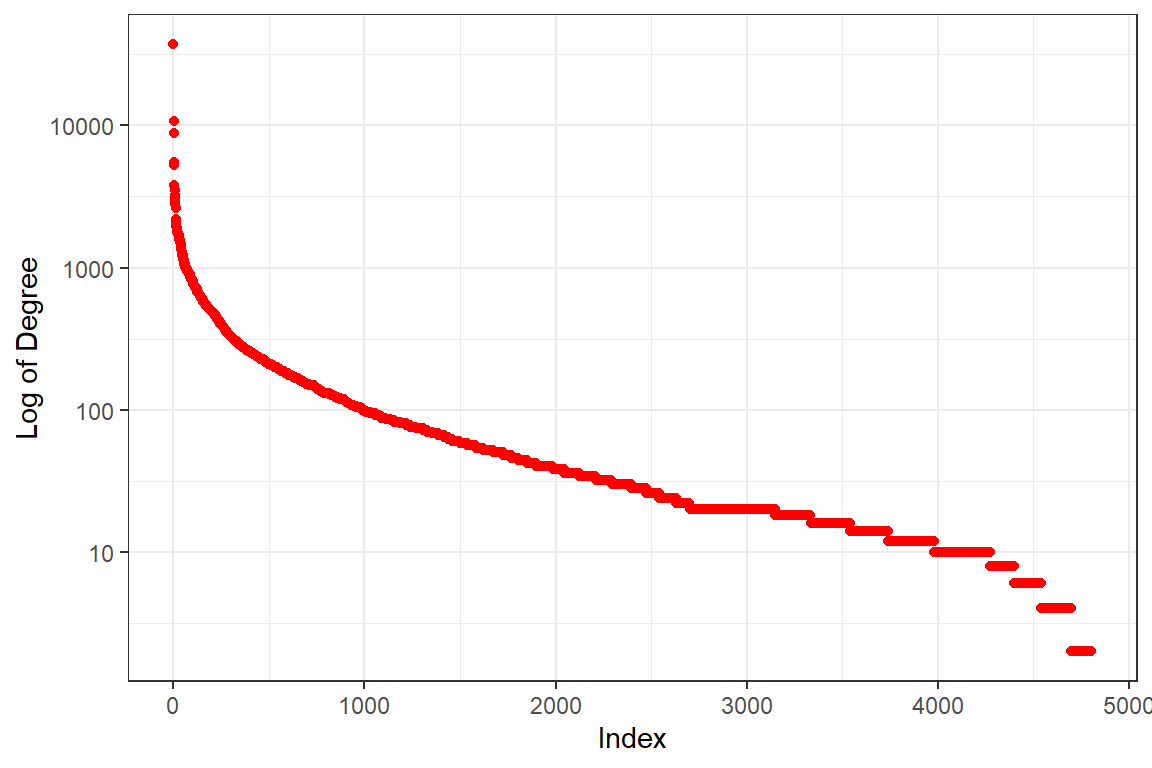
Figure 7.6: Plot of the degree distribution for Saheeh
Figure 7.6 looks similar to the tf-idf plot for Saheeh in Figure 2.14 from Chapter 2 - which indicates that the degree follows Zipf’s law, and hence is distributed following Power Law distributions. It shows the case where a very small number of words have a high degree of edges, whilst a very large number of words have an extremely small number of edges.
We show a simple demonstration what the degree means by printing the top twenty words ranked by its degree in the following texts, which is autogenerated by the codes written for this book:
allah, lord, people, day, earth, punishment, fear
messenger, believed, muhammad, truth, heavens, knowing, believers
life, disbelievers, fire, mercy, surely, moses
It is forming like a sentence, saying “Allah (the) Lord (of the) people, day (on) earth, punishment fear, messenger believed, Muhammad truth”. Actually, when we feed the texts into an unsupervised machine learning and recreate the texts, it will come out like what we have shown above.85 What it means is that the word with the highest probability is “allah” followed by “lord” and so on. This is probably why the challenge to come out with just one Surah, even a short Surah, is unmet until today.86 You must have the word “allah” or convey the meaning of oneness or Tauheed, which is impossible for the non-believers.
7.2.6 Clustering coefficients
There are many ways to compute clustering coefficients in a network, we will use the igraph method called transitivity(). The measure for the network transitivity is at 10.7%. This is a measure of the probability that given a node, the adjacent nodes (words) are connected. The number obtained here is extremely high. For most other real networks, the probabilities are extremely small; for example, the internet (0.003298%), World Wide Web (0.001412%), and E.coli metabolism (0.537055%). An implication of this finding is an indication of how “dense” the words are in the text, and almost no word is left without relations to other words.
For reference, we have seen examples of these clusterings earlier in Chapter 5 for Surah Yusuf and Chapter 6 for Surah Taa Haa.
7.2.7 Modularity
The modularity algorithm is used to find community structures or groupings of nodes and edges in large networks. In igraph, this is accomplished by applying the cluster_walktrap() function. However, this approach has some shortcomings, mainly because it relies on a random walk approach in finding communities, which is sensitive to the starting position and is used mainly in undirected graphs. For this purpose, we rely instead on the “modularity class” function of Gephi for calculations. The results are shown in Figure 7.7.
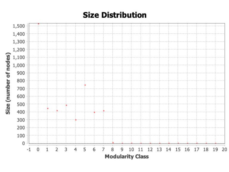
Figure 7.7: Modularity class
It is interesting to note that there are seven major modular classes with members of 300 or more, with the largest community having about 1,500 members.87 In fact, the smaller classes are with members of less than ten, and can be ignored (classes of 8 and above). The percentage of nodes within each class is as follows: 33.63% (one-third of the nodes), 17.87%, 15.68%, 9.58%, 8.33%, 7.42%, and 6.33% (from the first to the seventh).
In grouping terms, we can say that each modular class represents a certain “commonality”; if we want to understand what these commonalities are, then we dive deeper into each class and investigate inside the classes. Furthermore, we can set the resolution limit of the modularity measure, which allows us to break the classes into a more refined set. We leave this issue as a future research direction.
In this book, we will just show the visualizations of these classes (or groupings) to demonstrate the forms of shapes of the groups.
Figure 7.8 provides the total picture of the modularity classes within the network.
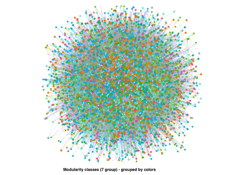
Figure 7.8: Modularity class by colors
Now let us check the structure of each of the various sub-groups. The largest grouping is shown in Figure 7.9, which has the same center as the entire network surrounded by words in the same modularity class. Figure 7.10 shows the second largest group, which has the same center as before but surrounded by another set of words. Figure 7.11 shows the third largest group is which has the same center as before but surrounded by another set of words.
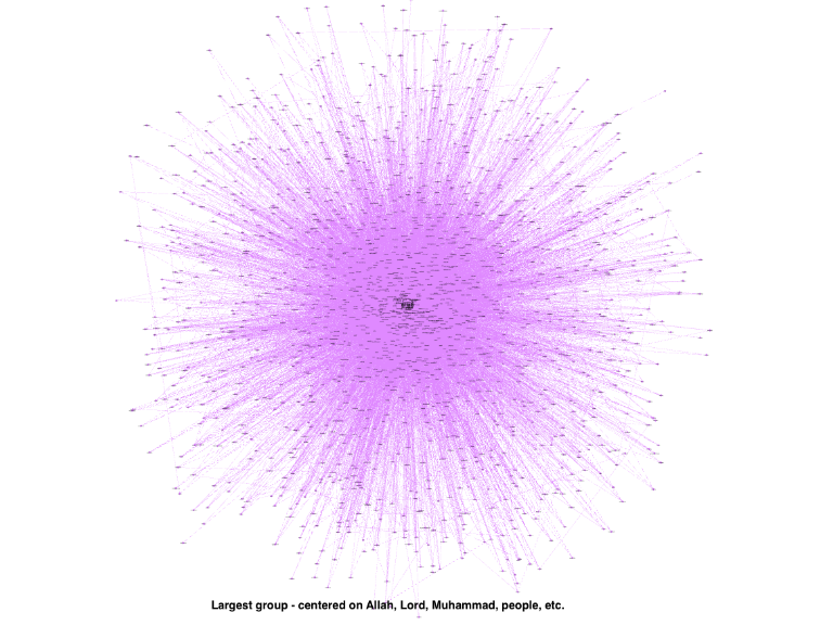
Figure 7.9: Network of largest clique
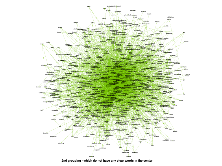
Figure 7.10: Network of second largest clique
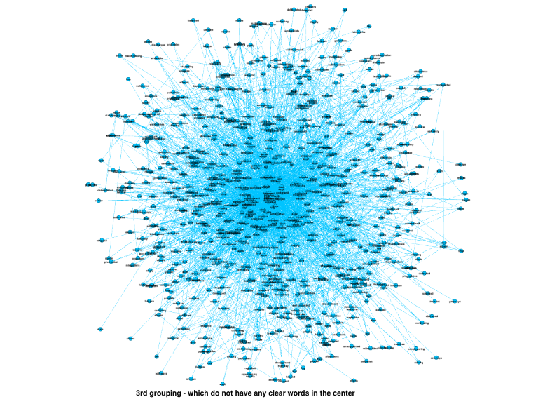
Figure 7.11: Network of third largest clique
We can move on to the fourth, fifth, and until the smallest grouping. The key point is what can we learn from these groups?
First, we want to observe how do the sub-networks look once we take them out of the main network. Do the sub-networks look and behave the same as the main network? Does the main network change when we take out a sub-network? All these questions relate to what is called the “scale-free” properties of a network. A scale-free network is resilient to changes within the network; when a clique is taken out, the clique’s properties are the same as the main network properties, while the properties of the network minus the clique also remain the same.
In another word, the network is structured in such a way that it behaves like a fractal - the large part is the combination of many small parts, while the small parts can exist by themselves, co-exist with other small parts, can be combined together and create a larger part, and so on. Fractal properties are resilient to “cascading failures” which is evident in most of nature’s physical properties.88
We can take the meaning of fractal properties into a much deeper context; for example, are the messages within the sub-network part of the composition of the main network? What happens to the messages in the main network when we take out a clique? Can we combine messages in two cliques and are the messages still coherent?
As an example, we can compile all the words within a clique and do a sentiment analysis on the subset of words, similar to what we have shown in Chapter 3. We can also weigh the sentiment scores against the position of the word within the sub-network, etc. Whatever meanings come out is subject to interpretation in terms of what they represent.
There are numerous ways to expand the current analysis, which is beyond the current introductory scope of this book. We will leave it for future work of Quran Analytics. For our purpose here, based on visual observations of the Figures 7.8, 7.9, 7.10, and 7.11, we can say that the network demonstrates some forms of “scale-free” (and fractal-like) properties. This is an important observation and provides leads for future exploration and analysis.
7.2.8 Betweenness
Betweenness measures the relative importance of words in connecting other words as the word in between. We compute the measures using the following codes:
btwnQ = betweenness(igphQ, v = V(igphQ), directed = TRUE,
                    weights = NULL, normalized = FALSE)
top_btwn = btwnQ[rev(order(btwnQ))]
Now let us use the results and rewrite the phrase as we have done earlier, using betweenness instead, as follows:
allah, lord, people, day, earth
punishment, fear, fire, believed, muhammad
created, evil, disbelievers, truth, messenger
women , moses , bring , hearts , surely
A comparison with words from the top degree, reveals some interesting observations. Except for the top few words, some other words changed their positions. This reflects the meaning of betweenness measures, that is some words appear more as a word in between two words, and lesser in terms of links.
7.2.9 Prestige centrality
Centrality measures refer to the centrality position of a word in the whole text. There are many ways to measure centrality, the simplest one being eigenvector centrality. This is the measure of the “importance” of a word. This is computed as the codes below:
evcentQ = eigen_centrality(igphQ)
top_evcent =evcentQ$vector
top_evcent = top_evcent[rev(order(top_evcent))]
We repeat the same exercise using the “prestige” as the rankings instead.
allah ,people ,lord ,earth ,fear
messenger ,day ,heavens ,knowing ,believed
punishment ,truth ,muhammad ,believers ,wills
merciful ,exalted ,mercy ,worship ,belongs
We do not intend to use the exercise here to interpret Al-Quran using the techniques used. However, for those who studied Al-Quran, some of the things shown here will start to make some sense of the direction of “knowledge” which can be extracted from using these measures of the network. So far, we have dealt only with the top-level words and have not dived deeper to lower-ranking texts (below 20), which might reveal many further insights. Again, we have to leave this for future work.
7.2.10 Summary
Summarizing all the statistical properties of the nodes of the network, we can say that all the important words (top features) have a high degree, betweenness, and prestige centrality within the network. The consistencies of these measures across these top features are very interesting in the sense that the first word, Allah is the topmost in all cases (the highest degree, highest prestige, the most betweenness, and also highest in all measures of centrality).
7.3 Dive into selected Surahs
The methods introduced in the previous section can be applied to a Surah as well as in performing comparisons between Surahs. Let us choose two intermediate-length Surahs, namely Al-Kahf (No. 18, 110 verses) and Maryam (No. 19, 98 verses). There are a few approaches we could take:
- understanding the total network of the texts (tokens) in the Surah;
- understanding the “topics” of the Surah.
First, we will plot the network and obtain summary statistics.
kahf = quran_en_sahih[grep("Al-Kahf",quran_en_sahih$surah_title_en),]
kahf_toks <- kahf$text %>%
    tokens(remove_punct = TRUE) %>%
    tokens_tolower() %>%
    tokens_remove(pattern = stop_words$word, padding = FALSE)
dfm_kahf = dfm(kahf_toks)
fcmKahf <- fcm(kahf_toks,
             context = "window",
             tri = FALSE)
igphKahf = quanteda.textplots::as.igraph(fcmKahf)
degKahf = degree(igphKahf, v = V(igphKahf),
                   mode = "total", loops = TRUE,
                   normalized = FALSE)
top_degreeKahf = degKahf[rev(order(degKahf))]
btwnKahf = betweenness(igphKahf, v=V(igphKahf), directed = TRUE,
                         weights = NULL, normalized = FALSE)
top_btwnKahf = btwnKahf[rev(order(btwnKahf))]
evcentKahf = eigen_centrality(igphKahf)
top_evcent =evcentKahf$vector
top_evcentKahf = top_evcent[rev(order(top_evcent))]
featKahf <- names(topfeatures(fcmKahf, 50))fcm_select(fcmKahf, pattern = featKahf) %>%
textplot_network(min_freq = 0.5,
edge_color = "steelblue",
edge_alpha = 0.5,
edge_size = 2,
vertex.size = 1)+
theme(plot.title = element_text(hjust = 0.5),
plot.background = element_rect(color = "black"))+
labs(title = 'Network of Top 50 Words in Surah Al-Kahf',
subtitle = " ")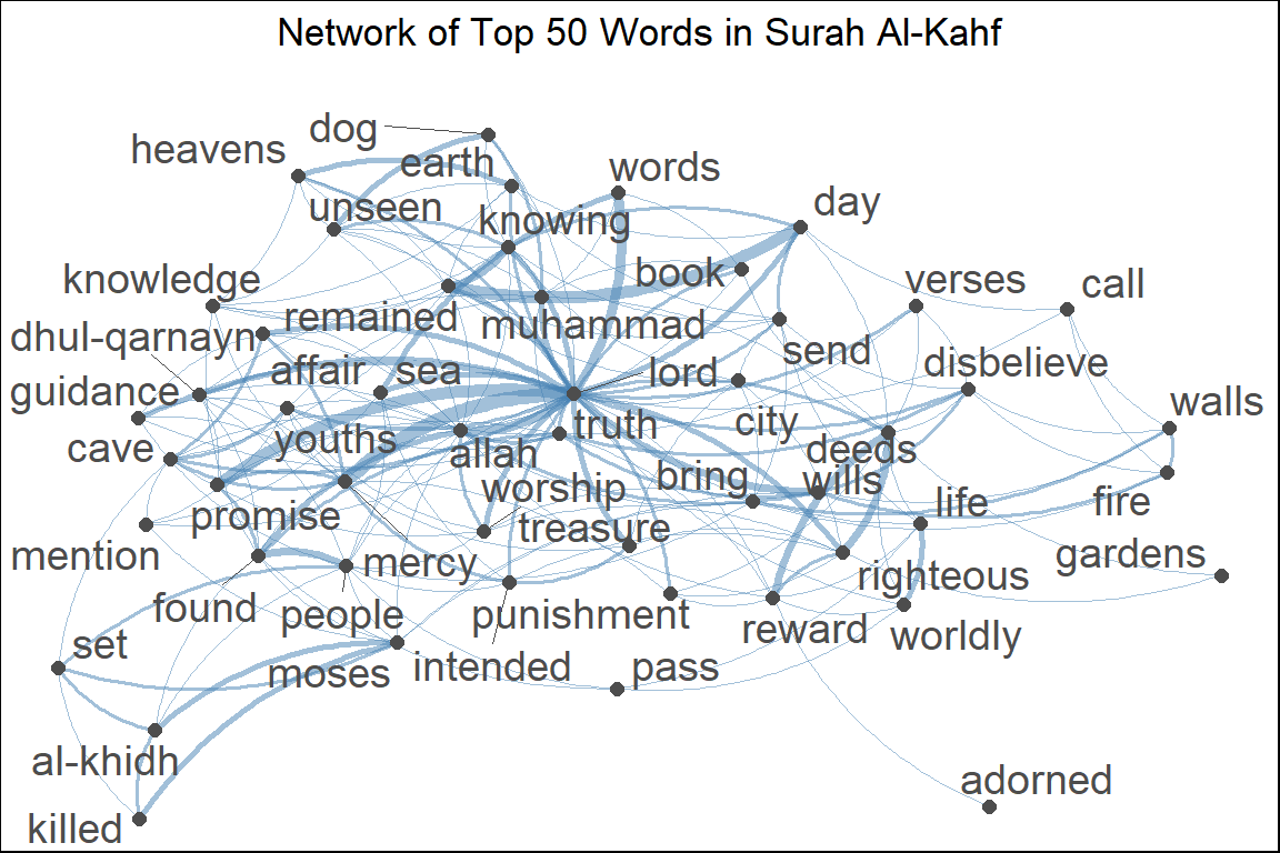
Figure 7.12: Network of top 50 words in Surah Al-Kahf
maryam = quran_en_sahih[grep("Maryam",quran_en_sahih$surah_title_en),]
maryam_toks <- maryam$text %>%
    tokens(remove_punct = TRUE) %>%
    tokens_tolower() %>%
    tokens_remove(pattern = stop_words$word,
                  padding = FALSE)
dfm_maryam = dfm(maryam_toks)
fcmMaryam <- fcm(maryam_toks,
             context = "window",
             tri = FALSE)
igphMaryam = quanteda.textplots::as.igraph(fcmMaryam)
degMaryam = degree(igphMaryam, v = V(igphMaryam),
                   mode = "total", loops = TRUE,
                   normalized = FALSE)
top_degreeMaryam = degMaryam[rev(order(degMaryam))]
btwnMaryam = betweenness(igphMaryam, v=V(igphMaryam), directed = TRUE,
                         weights = NULL, normalized = FALSE)
top_btwnMaryam = btwnMaryam[rev(order(btwnMaryam))]
evcentMaryam = eigen_centrality(igphMaryam)
top_evcent =evcentMaryam$vector
top_evcentMaryam = top_evcent[rev(order(top_evcent))]

featMaryam <- names(topfeatures(fcmMaryam, 50))fcm_select(fcmMaryam, pattern = featMaryam) %>%
textplot_network(min_freq = 0.5,
edge_color = "tomato",
edge_alpha = 0.5,
edge_size = 2,
vertex.size = 1)+
theme(plot.title = element_text(hjust = 0.5),
plot.background = element_rect(color = "black"))+
labs(title = 'Network of Top 50 Words in Surah Maryam',
subtitle = " ") 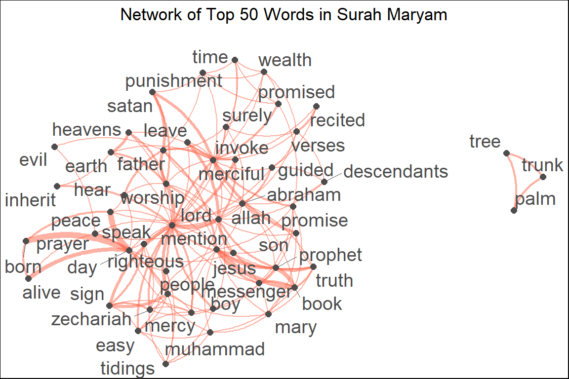
Figure 7.13: Network of top 50 words in Surah Maryam
For both Surahs, as shown in the figures, the most prominent word at the center is “lord”; however the surrounding topics are different. In Al-Kahf words such as “cave”, “youth”, “al-khidh”, “moses” emerge, while in Surah Maryam “merciful”, “jesus” appear.
The summary statistics are tabulated in the Table:
| Statistics | Surah Al-Kahf | Surah Maryam |
|---|---|---|
| Nodes | 506 | 326 |
| Edges | 5,516 | 2,838 |
| Average degree | 21.8 | 17.41 |
| Diameter | 7 | 7 |
| Average Path Length | 3.06 | 3.24 |
| Size of largest component | 504 | 315 |
| Transitivity | 0.28 | 0.33 |
The table above reveals that the network characteristics of both Surahs are not far from each other. Despite Al-Kahf being a bit longer, which results in more nodes and edges, the diameter, average distance to the center, are all about the same.
Now let us try to get some ideas regarding the thematic subjects of both Surahs, from the three elements of measures: degree, clustering, and betweenness.
| Surah Al-Kahf | Text |
|---|---|
| By degree | lord ,allah ,people ,moses ,found ,earth ,mercy |
| deeds ,day ,remained ,bring ,truth ,cave ,knowing | |
| righteous ,reward ,sea ,muhammad ,al-khidh ,send | |
| By betweenness | lord ,allah ,moses ,people ,earth ,reward ,day |
| bring ,gardens ,deeds ,cave ,beneath ,remained ,found | |
| dog ,muhammad ,send ,affair ,truth ,time | |
| By prestige centrality | lord ,allah ,mercy ,promise ,remained ,words ,knowing |
| day ,wills ,righteous ,affair ,truth ,deeds ,exhausted | |
| worship ,cave ,muhammad ,sea ,associate ,guidance |
One way to interpret the keywords is that the main keywords are (in the order of): “lord”, “allah”, then by the number of mentions: “people”, by between the subjects: “moses”, and by the prestige of mention: “mercy”.
| Surah Maryam | Text |
|---|---|
| By degree | lord ,merciful ,allah ,day ,mention ,father ,people |
| worship ,prophet ,surely ,abraham ,book ,prayer ,boy | |
| jesus ,verses ,punishment ,peace ,promised ,earth | |
| By betweenness | lord ,merciful ,allah ,day ,died ,alive ,surely |
| father ,people ,worship ,prayer ,abraham ,hear ,brought | |
| mention ,earth ,jesus ,speak ,angel ,destroyed | |
| By prestige centrality | lord ,allah ,worship ,people ,merciful ,day ,mention |
| sign ,invoke ,prophet ,jesus ,father ,leave ,book | |
| unhappy ,zechariah ,mercy ,boy ,peace ,abraham |
One way to interpret the keywords is that the main keywords are (in the order of): “lord”, then by the number of mentions: “merciful”, by between the subjects: “merciful”, and by the prestige of mention: “worship”.
7.4 Word collocations statistical method
In this section we will take another approach to the computations of word collocations, namely using various statistical tools. Most of these tools utilize what is called “distance measures”, which mathematically is the calculation relative statistical scoring of multi-word expressions. The multi-word can be set to two (i.e. bigrams) or three (i.e. trigrams), and so on, depending on the objective of the analysis.
The function we can apply is textstat_collocations() from quanteda. Here we show how this function is applied and what the results meant(Blaheta and Johnson 2001).
What is the most important two-word sequence in Surah Al-Kahf?
tscKahf = kahf_toks %>% quanteda.textstats::textstat_collocations(method = "lambda", size = 2,
                        min_count = 1,smoothing = 0.5,tolower = TRUE)
tscKahf[tscKahf$count == max(tscKahf$count),]$collocation
## [1] "righteous deeds" "worldly life" "heavens earth" "lord knowing"What is the most important three-word sequence in Surah Al_Kahf?
tscKahf = kahf_toks %>%
              textstat_collocations(method = "lambda", size = 3,
                        min_count = 1,smoothing = 0.5,tolower = TRUE)
tscKahf[tscKahf$count == max(tscKahf$count),]$collocation
## [1] "mercy prepare affair" "believed righteous deeds"What is the most important two-word sequence in Surah Maryam?
tscMaryam = maryam_toks %>%
              textstat_collocations(method = "lambda", size = 2,
                        min_count = 1,smoothing = 0.5,tolower = TRUE)
tscMaryam[tscMaryam$count == max(tscMaryam$count),]$collocation
## [1] "mention book"What is the most important three-word sequence in Surah Maryam?
tscMaryam = maryam_toks %>%
              textstat_collocations(method = "lambda", size = 3,
                        min_count = 1,smoothing = 0.5,tolower = TRUE)
tscMaryam[tscMaryam$count == max(tscMaryam$count),]$collocation
## [1] "peace day born" "day raised alive" "day born day" "trunk palm tree"The results in the exercises indicate that out of all possible collocations (bigrams for two-word phrases and trigrams for three-word phrases), these resulting phrases rank highest in the entire text (i.e. the chosen Surah). They stood out as the most “outstanding phrases” which explain the subject of the texts (i.e. Surah). Whether the results make any meaningful sense or not is a subject of the interpretation of the texts (i.e., translated text of Al-Quran).
As a comparison, we will do the same for Surah Maryam for Yusuf Ali (instead of Saheeh as done before). Will we get the same answer? (We will show only the results since the codes follow the same steps).
quranEY <- quran_en_yusufali %>%
             select(surah_id,
                    ayah_id,
                    surah_title_en,
                    surah_title_en_trans,
                    revelation_type,
                    text,
                    ayah_title)
maryamEY = quranEY[grep("Maryam",quranEY$surah_title_en),]
maryamEY_toks <- maryamEY$text %>%
    tokens(remove_punct = TRUE) %>%
    tokens_tolower() %>%
    tokens_remove(pattern = stop_words$word,
                  padding = FALSE)
What are the most important two-word sequences in Surah Maryam in Yusuf Ali?
tscMaryamEY = maryamEY_toks %>%
                textstat_collocations(method = "lambda", size = 2,
                    min_count = 1,smoothing = 0.5,tolower = TRUE)
tscMaryamEY[tscMaryamEY$count == max(tscMaryamEY$count),]$collocation
## [1] "allah gracious"What are the most important three-word sequences in Surah Maryam in Yusuf Ali?
tscMaryamEY = maryamEY_toks %>%
                textstat_collocations(method = "lambda", size = 3,
                        min_count = 1,smoothing = 0.5,tolower = TRUE)
tscMaryamEY[tscMaryamEY$count == max(tscMaryamEY$count),]$collocation
## [1] "mention book story"We can see that Yusuf Ali’s translations will give a different phrase. In fact, if we go deeper into phrases of slightly lower ranking, some of the phrases do match.
7.5 Word keyness comparisons
If we want to compare the keywords of one Surah against another Surah, we can use the keyness statistical measures. In quanteda we can use textstat_keyness() function and also textplot_keyness() for plotting the results. Let us compare prominent keywords in Surah Al-Kahf versus Maryam. This is shown in Figure 7.14.
kahf_1 = kahf %>% pull(text) %>% str_flatten()
maryam_1 = maryam %>% pull(text) %>% str_flatten()
kahf_maryam = kahf_maryam = rbind(kahf_1,maryam_1)

corp = corpus(kahf_maryam,
              docvarsz = c("kahf","maryam"))
names(corp) = c("kahf","maryam")

dfmat2 <- dfm(corp,
              # groups = "surah",
              remove = stop_words$word,
              remove_punct = TRUE)
tstat2 <- textstat_keyness(dfmat2, target = "kahf", measure = "lr")
textplot_keyness(tstat2, color = c("steelblue", "tomato"), n = 20)+
  labs(title = "Keyness For Surah Maryam and Surah Al-Kahf")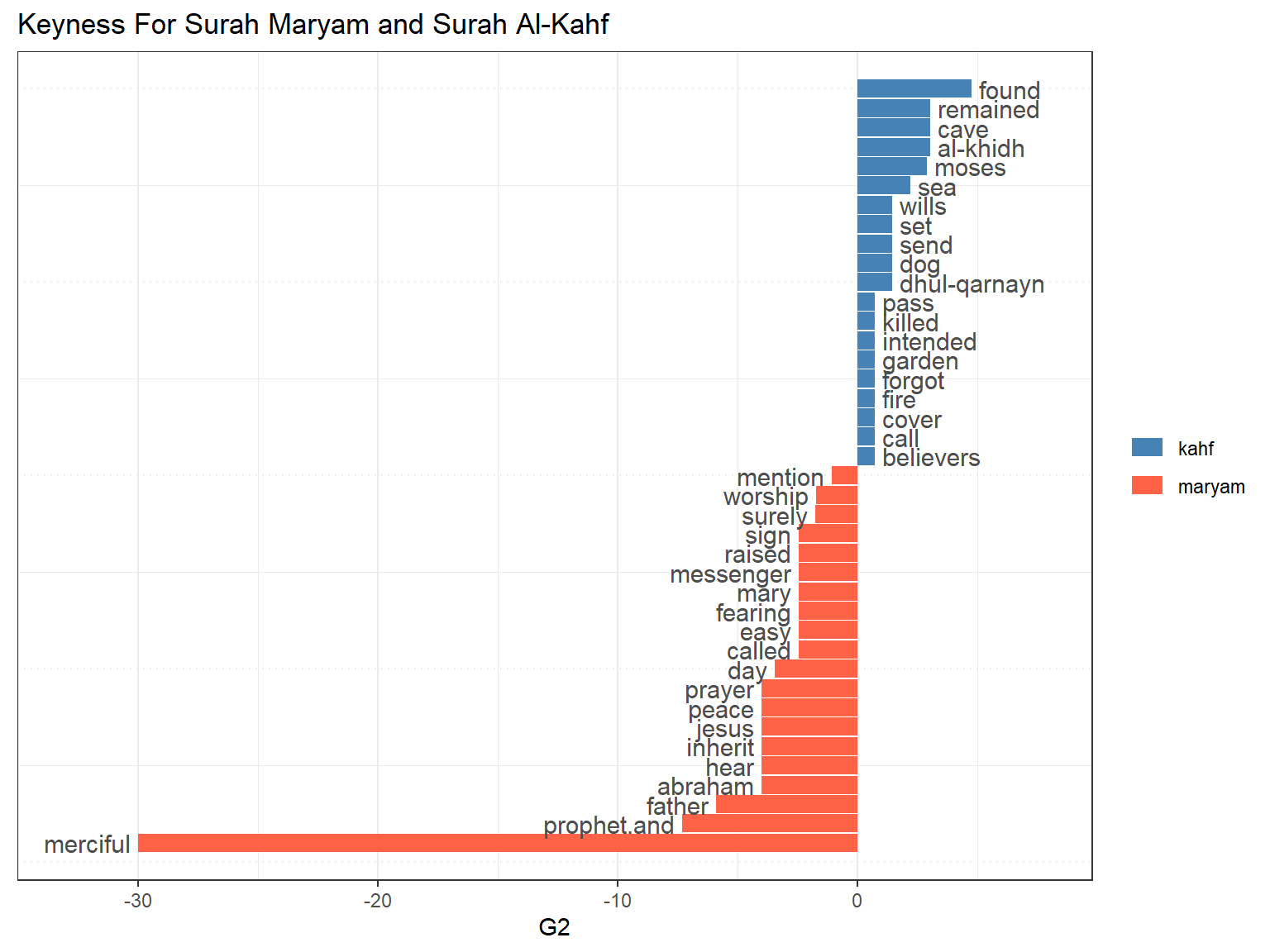
Figure 7.14: Keyness plot for Surah Maryam and Al-Kahf
The keyness plot shows and confirms what is known about the two Surahs. In Surah Al-Kahf, the word “found” relates to the cave-dwellers and al-khidh (Khidir) as well as Dhul-Qarnayn. In Surah Maryam, the key message is “merciful”, an attribute of Allah, and Maryam (Mary) and her son Isa (AS) as signs of His mercy.
7.6 Lexical diversity and dispersion
Lexical diversity is a measure of how each sentence adds to the lexical variety in terms of its addition to the vocabulary within a corpus. Let us make a comparison between Surah Al-Kahf and Surah Maryam, by calculating textstat_lexdiv() scores and plotting the results side by side.
kahf_lexdiv = textstat_lexdiv(dfm_kahf, measure = "all")
maryam_lexdiv = textstat_lexdiv(dfm_maryam, measure = "all" )
p1 = ggplot() + geom_point(aes(x = 1:nrow(kahf_lexdiv),
                               y = kahf_lexdiv$R),
                               color = "steelblue",
                           show.legend = FALSE) + ylim(0,5)+
                labs(x = "Verse", y = "Lexical Diversity Score",title = "Surah Al-Kahf")
p2 = ggplot() + geom_point(aes(x = 1:nrow(maryam_lexdiv),
                               y = maryam_lexdiv$R),
                               color = "tomato",
                               show.legend = FALSE) + ylim(0,5)+
                labs(x = "Verse", y = "Lexical Diversity Score",title = "Surah Maryam")
cowplot::plot_grid(p1,p2, nrow = 1,align = "v")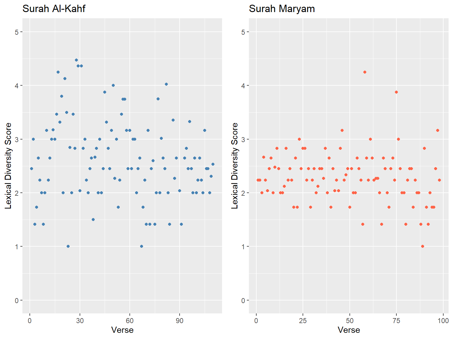
Figure 7.15: Lexical diversity scores for Surah Al-Kahf and Maryam
We can observe from Figure 7.15 that the verses in Surah Al-Kahf are much more diverse in their lexical diversity, throughout the Surah; whereas Surah Maryam’s later verses (after verse 50) show more variety. What this implies is that the vocabulary structure in the verses of Surah Al-Kahf is different from Surah Maryam.
Another approach of comparison is called key words in context or kwic lexical dispersion plot. Note that “text1” to “text110” is from Surah Al-Kahf and the rest (“text111 to”text208”) are from Surah Maryam.
First, let us apply it to the word “Allah” and “Lord”.
textplot_xray(kwic(corp, pattern = "allah"), kwic(corp, pattern = "lord"),
              scale = "absolute") +
              aes(color = keyword) +
              scale_color_manual(values = c("darkblue", "darkred")) +
              theme(legend.position = "none",
                    strip.background = element_rect(color = "black", size = 1))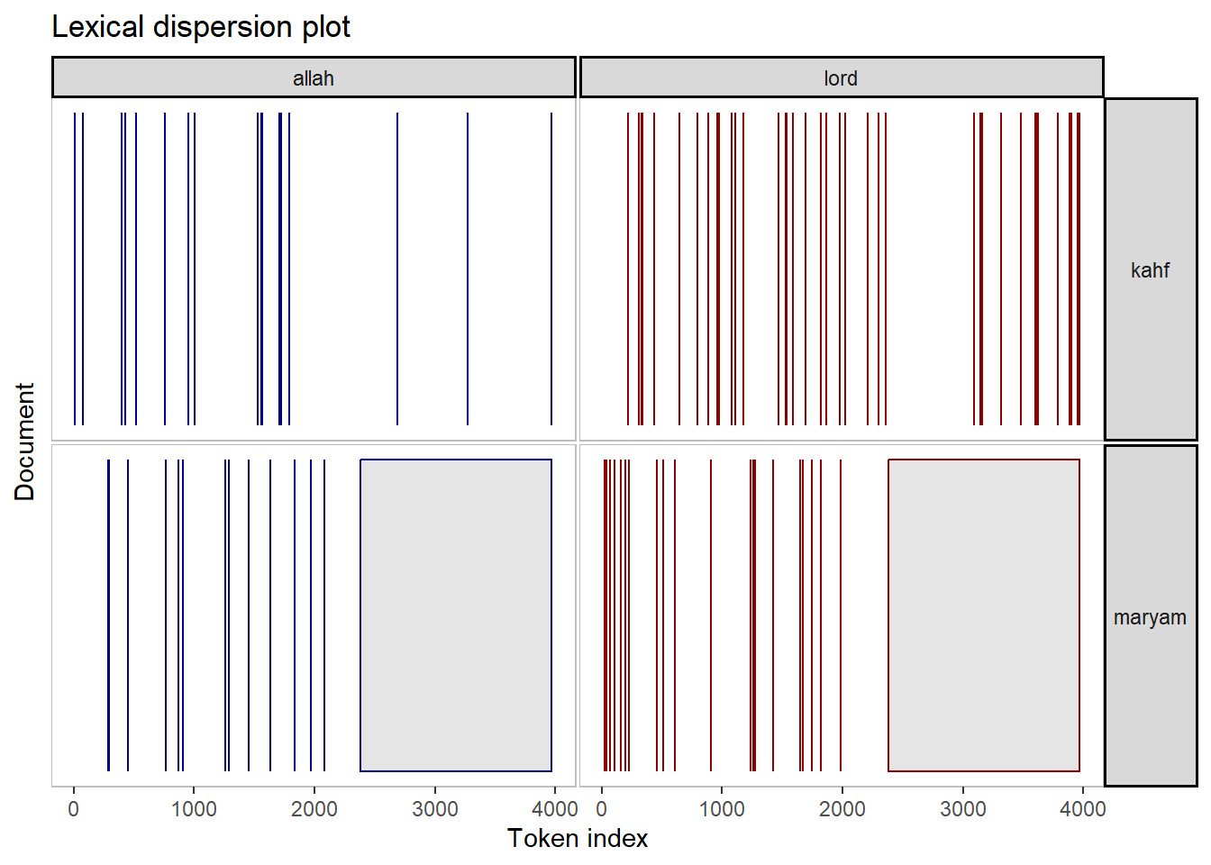
Figure 7.16: Keyword in context (kwic) plot for Surah Maryam and Al-Kahf for the word ‘Allah’ and ‘Lord’
The plots in Figure 7.16 display the frequency of the selected keyword and its appearance within the various verses (“texts”). Lexical dispersion demonstrates the richness of emphasis of the whole document regarding the message, via frequencies of occurrence relative to the sentences (verses) within the document.
The word “Allah” appears lesser than “Lord” in both Surahs. There are some occasions when “Allah” is mentioned, “Lord” is also mentioned (i.e. the lines where both blue and red dots exist). However, there are many verses in which “Lord” is mentioned without the mention of the word “Allah” (lower parts of the plot).
What the exercise does is to get some sense into why, lexically, certain words appear in some verses (or Surahs), and do not appear in some other verses (or Surahs). The explanation of why there are patterns of appearance is a subject of the interpretation of Al-Quran. The method we use here is only a tool to detect and visualize the patterns.
7.7 Viewing the network as dendrogram
We would like to end by presenting another tool that is useful for viewing a large network of co-occurrence data as we have been dealing with in the previous sections. The dendrogram is useful to view “clustering” or “grouping” of the networks using algorithms such as fast_greedy or cluster_edge_betweenness as discussed in Chapter 5.
Let us show the results for both Surahs.
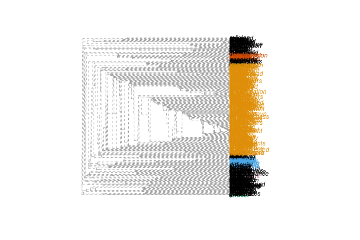
Figure 7.17: Dendrogram for clusters in Surah Al-Kahf
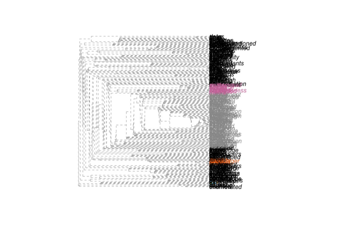
Figure 7.18: Dendrogram for clusters in Surah Maryam
We can see from Figure 7.17 and Figure 7.18 that there are clusterings or groupings in the cooccurrences words; in fact there are about three large groupings in Surah Al-Kahf and Surah Maryam. We can extract out the data for the groupings and do further analysis as needed and required. We leave the subject as it is for our work here.
7.8 Words similarity in verses
The concept of similarity in texts in NLP applies to sentences or in our case verses. How similar are any two verses in a set of verses, such as a Surah? Or how similar are verses from one Surah compared to verses from another Surah? This is like posing a question: does a verse contains similar words (not necessarily in the same order) with another given verse?
In linear algebra, the measure is the dot product of two vectors of not necessarily similar length, normalized to the product of their Euclidean norms, called cosine similarity (\(cosine_{sim}(x,y) = \frac{x.y}{|x|.|y|}\)). Similar measure is called jaccard similarity, which is the measure of set similarity instead of dot product (\(jaccard_{sim}(a,b) = \frac{|a \cap b}{|a \cup b|}\)).
This can be applied using the textstat_simil() function in quanteda.
tstcor_kahf = textstat_simil(dfm_kahf, y = NULL,
               margin = "documents",
               method = "correlation")
tstcor_kahf = as.data.frame(tstcor_kahf)
tstcor_kahf = tstcor_kahf %>% filter(correlation > 0)
tstcos_kahf = textstat_simil(dfm_kahf, y = NULL,
               margin = "documents",
               method = "cosine")
tstcos_kahf = as.data.frame(tstcos_kahf)
tstjac_kahf = textstat_simil(dfm_kahf, y = NULL,
               margin = "documents",
               method = "jaccard")
tstjac_kahf = as.data.frame(tstjac_kahf)
ggplot() +
  geom_point(aes(x = c(1:length(tstcor_kahf$correlation)), y = tstcor_kahf$correlation), color = "red") +
  geom_point(aes(x = c(1:length(tstcos_kahf$cosine)), y = tstcos_kahf$cosine), color = "blue") +
  geom_point(aes(x = c(1:length(tstjac_kahf$jaccard)), y = tstjac_kahf$jaccard), color = "#3B9D47") +
  labs(x = "Edges", y = "Similarity Score",
       title = "Verses Similarity for Surah Al-Kahf",
       subtitle = "Using <span style = 'color: red;'>Correlation</span>, <span style = 'color: blue;'>Cosine</span> and <span style = 'color: #31783A;'>Jaccard</span> measures")+
  theme(plot.subtitle = element_markdown())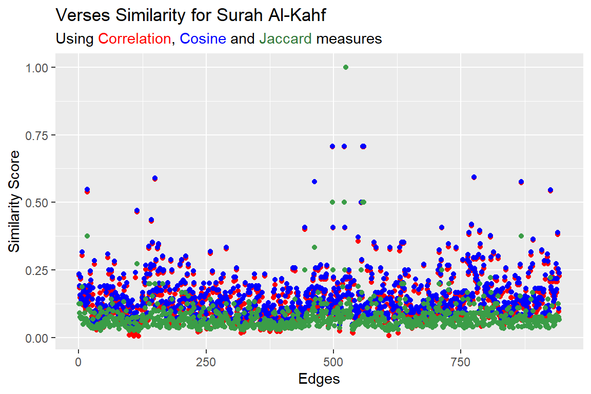
Figure 7.19: Verses similarity for Surah Al-Kahf using correlation, cosine and jaccard measures
Figure 7.19 shows the plot for three measures namely correlation (red), cosine (blue), jaccard (green). Two verses are 100% similar textually, word-for-word, and a good number with a similarity score above 25% (i.e. more than a quarter of the words). What do all these numbers mean depends on how interpretations are made; for example, it can be said that these verses explain each other.
tstcos_kahf$document1 = str_replace(tstcos_kahf$document1,"text","")
tstcos_kahf$document2 = str_replace(tstcos_kahf$document2,"text","")
igph_kahfcos = graph_from_data_frame(tstcos_kahf %>%
                                       filter(cosine > 0.25))
ggraph(igph_kahfcos, layout = "kk") +
  geom_edge_link(aes(width = cosine, edge_alpha = cosine),
                     edge_color = "steelblue") +
  geom_node_point(size = 0.1, shape = 1, color = "black") +
  geom_node_text(aes(label = name), col = "black", size = 4)+
  theme_bw()+
  labs(title = "Verses with High Similarity for Surah Al-Kahf")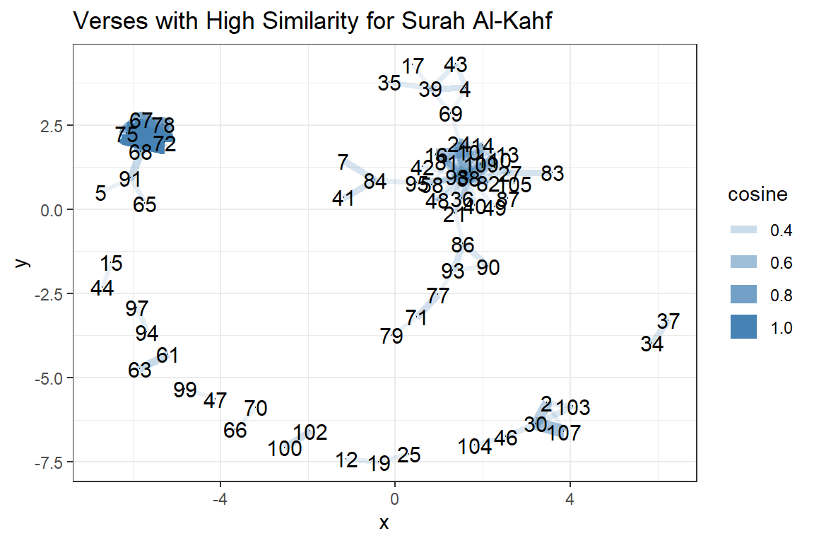
Figure 7.20: Verses with high similarities for Surah Al-Kahf
The best way is to view them as an igraph plot using ggraph (as discussed in the previous chapter). Figure 7.20 shows clusters of verses that are linked. If we check further, the verses around v65 to v78, are repeated conversations between Moses and Khidh. The other cluster surrounding v38, is about the story of the cave dwellers. What we have shown is how statistical tools in NLP are used to find related sentences (or verses) in a large text (if we apply them to the entire translation).
For completeness, we will show similar plots for Surah Maryam (Figures 7.21 and 7.22). We leave the readers to check why the verses are linked in this manner for the Surah.
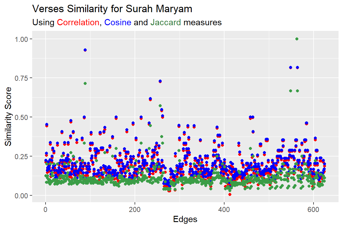
Figure 7.21: Verses similarity for Surah Maryam using correlation, cosine and jaccard measures
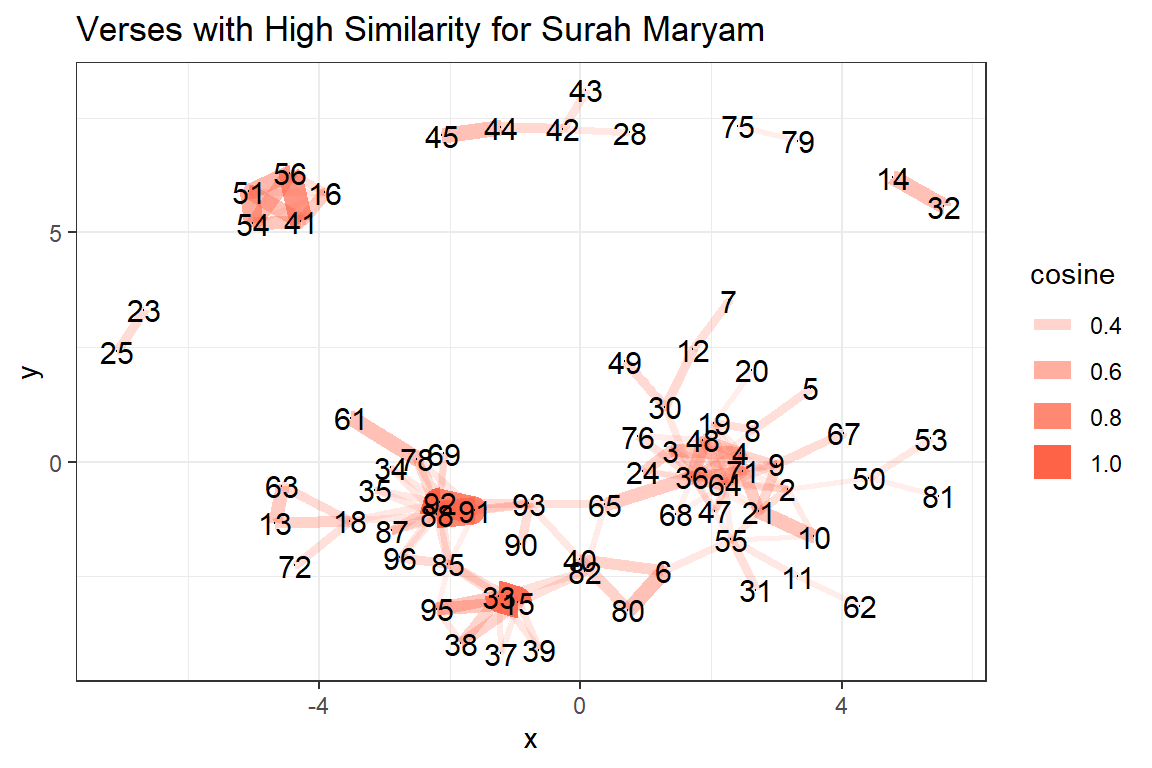
Figure 7.22: Verses with high similarities for Surah Maryam
7.9 Words dissimilarity in verses
The inverse of the concept of similarity is the concept of distance in text. How different are any two verses in a set of verses, such as in a Surah will be?
In linear algebra, the measure is the simple Euclidean distance of two vectors.89 There are few options in textstat_dist() function in quanteda besides euclidean, like minkowski90 and manhattan91. We will use manhattan, because it is the most amplified version of distance.
tstdis_kahf = textstat_dist(dfm_kahf, y = NULL,
               margin = "documents",
               method = "manhattan")
tstdis_kahf = as.data.frame(tstdis_kahf)
ggplot() + geom_point(
              aes(x = c(1:nrow(tstdis_kahf)),
                  y = scale(tstdis_kahf$manhattan, scale = F)),
              color = "#54B660") +
              labs(x = "Edges", y = "Distance Score",
                   title = "Verses Distance for Surah Al-Kahf",
                   subtitle = "Using Manhattan Measures")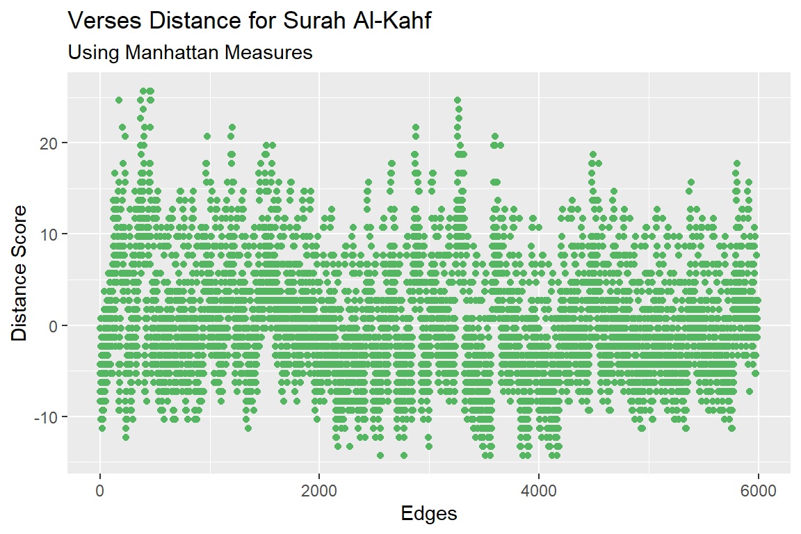
Figure 7.23: Verses distance for Surah Al-Kahf using manhattan measures
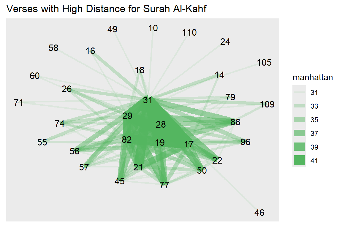
Figure 7.24: Verses with high distances for Surah Al-Kahf
Figures 7.23 and 7.24 guide us to check why verse 45 is very different than verse 29. Many similar exercises are possible by extracting out the data (as plotted) and analyzing them in whichever ways a researcher deems suitable.
The methods of similarity and distance are different from sentiment scoring in Chapter 3. Here the focus is on similar words existing in two different sentences. The more the similarity is, the higher the cosine (or other similarity measures) is. If there is no word matching, then the higher the distance is (measured by euclidean or manhattan scores).
We will not repeat the exercises for Surah Maryam and we also will not do similar exercises on Yusuf Ali for brevity. We leave it for readers’ own exercise using the R codes enclosed together with the book.
7.10 Summary
We have demonstrated using the quanteda package how to work with various NLP tasks for the Saheeh English translation of Al-Quran. The applications can be extended to include all other versions of English translations and non-English translations using the methods shown. One point to emphasize is, we have used tools that are language-model independent. None of the methods shown require any assumptions of pre-built models of a language (except for the use of pre-built stopwords). These are non-parametric methods that we promoted as the basis for unsupervised learning methods, which is a fast-developing area in the applications for NLP tasks.
We have provided only glimpses of what are the possible tools and methods, which a researcher of Quran Analytics can take further. We provide some suggestions here.
Expand the usage of the tools to develop methods of analysis based on the objective of linguistics and analytical studies for translations of Al-Quran and benchmark it against linguistic models (for the selected language) and against the original text of Al-Quran.
Network models of texts are versatile and expandable in many directions, as a non-parametric approach and application of graph theory or network science algorithms.
Language, which consists of words as one of its basic elements, can be viewed as a system or systems. Network models of language allow us to study language from the perspective of network dynamics and systems theory.
Tools of NLP in R such as quanteda are extremely versatile because they do not force us to make prior underlying assumptions. We can just let the statistical results and visuals open up interesting questions that we can explore further.
7.11 Further readings
quanteda package documentation (https://quanteda.io).
quanteda manual and guides (Benoit et al. 2018)
Ban, K., Meštrović, A., and Martincic-Ipsic, S. (2014). Initial comparison of linguistic networks measures for parallel texts (Ban, Meštrović, and Martincic-Ipsic 2014).
References
Lexical semantics, Oxford research encyclopedias; https://oxfordre.com/linguistics/view/10.1093/acrefore/9780199384655.001.0001/acrefore-9780199384655-e-29↩︎
For general reference, readers should refer to the quanteda documentation and tutorials at https://quanteda.io/index.html↩︎
We do not enclose the plots here to save space. Readers can repeat the same exercise using the enclosed code to check the results for themselves.↩︎
The figure is obtained from Gephi; since plotting a large network of this size is not efficient in R↩︎
Please refer to https://en.wikipedia.org/wiki/Watts–Strogatz_model, for a quick guide.↩︎
This is a very important phenomenon that requires deeper interpretations. Just imagine web pages of the Internet, whereby every page is directly or indirectly connected to every other page on the network. We know that this is not true in the case of the Internet.↩︎
Tests using unsupervised learning LSTM Neural Network model was done by the first author; the results of which are not fully ready for publication at the time of this writing.↩︎
Refer to verse 2:23↩︎
Modularity algorithm is dependent on its setting of resolution limits, which determines how small the communities we want to detect. In our case here we set it to 1, which is the standard limit.↩︎
For more on fractal properties, please refer to https://en.wikipedia.org/wiki/Fractal.↩︎